Map Digitization |
  
|
Map Digitization |
|
You start this module by selecting "Maps" from the main REP window or by choosing Maps | Maps digitisation from the drop-down menu on the same main REP window.
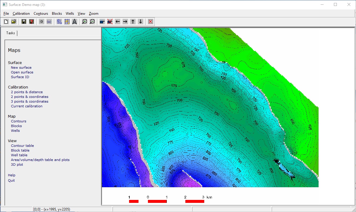
You start with an image of a contour map, digitise it using the mouse, and create a surface file (srf extension). The area/depth table stored in the srf file can be loaded into the GRV entry section of a prospect/file calculation.
The digitisation process is simple: first you must calibrate the image using the scale bar (so it is important that this is shown on the map image). Then you trace round each contour with the mouse. With simple maps it is usually not necessary to digitise all the contours in a first pass. Later on you can always come back and trace around some more, so get more accuracy if the problem warrants it.
Currently supported image formats are bmp, jpg (jpeg), pcx, tif, and tga. There is a limit to how large an image can be, depending on the capabilities of your PC. If REP fails to load the image, try using a graphics package (e.g PaintShop Pro) to reduce the file size. If you don't have access to a suitable graphics package, send it to support@logicomep.com and we will convert it for you.
It is best to place the image file in the same folder as you will put the prospect and consolidation files when you make the main REP calculations.
The topics in the section are:
The main tasks are shown in the left panel. All these and extra facilities are available from the top menu.
First you need to specify the image file you wish to digitise:
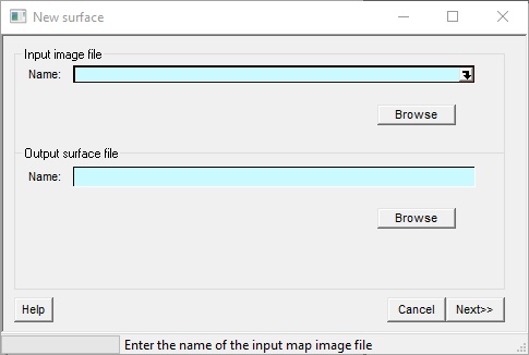
Input image file |
Specify the image file. Browse to it, or choose a recently used one from the drop down |
Output surface file |
The is the same of the .srf file you are going to create. By default it takes the same name and location as the image file, but you can change it of course. |
You can load up a previously created surface file. ("Open surface"). The is a similar dialog to that shown above, with the order of the two files reversed.
If the image file is successfully loaded it is shown in the main window.
When you have loaded an image, you will see the Surface definition screen. Here you give the surface a name and a qualifying comment.
The four units required for calculations are depth, area, distance and volume.
You must also enter the surface crest. This is the highest point on the surface, for which the associated contour area is, by definition, zero.
The contour interval (depth difference between contours) and the first contour can be entered here. These are useful entries but it is not absolutely necessary to get them right. You always confirm the depth of any contour you digitise.
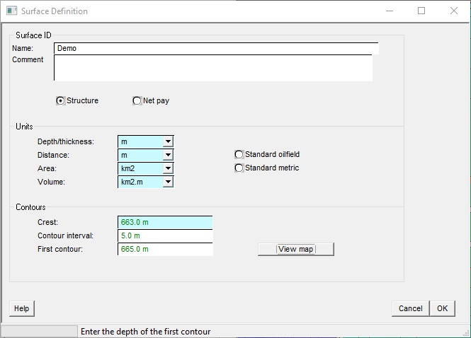
Surface ID |
|
Name |
Choose a name for the Surface |
Comment |
Use this field for any relevant comments |
Structure/net pay |
If you are digitising a new pay map (which is definitely not recommended, by the way) check it here. |
Units |
|
Depth |
Choose the unit for depth |
Distance |
Choose the unit for distance |
Area |
Choose the unit for area |
Volume |
Choose the unit for volume |
Contours |
|
Crest |
Enter the depth of the highest point on the structure (i.e. where area=0) |
Contour Interval |
Enter the interval between contours |
First Contour |
Enter the first contour |
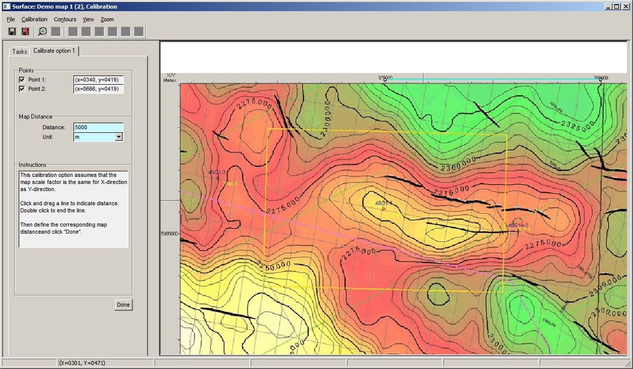
Before doing any digitising, you must calibrate the map. Calibration is an essential step, and you need to get it right.
There are three methods, the most common of which is "2 points & distance".
i.Click on two points and give the corresponding map distance.
ii.Click on two points and give the corresponding map co-ordinates.
iii.Click on three distinct (non-linear) points and give the corresponding map co-ordinates.
Co-ordinates are given in UTM style - usually metres.
You can recalibrate at any time.
The first two options presume that the map scale factor is the same in both the x- and y-directions. By using three points the third option allows for different scale factors in the x- and y- directions. This might happen if you have used your phone to photograph the map and haven't got it lined up perfectly, so that there is some distortion.
Select the appropriate method from the task menu. The process is similar for each method, and instructions are given on the dialog.
Left-click the mouse cursor at the first calibration point, then left click at the second. If you are doing three points, left-click again at the third, Double click to end.
You can click and drag the line end points to get your calibration spot-on. Zooming in can be useful.
Finally, enter the corresponding distance/coordinate information. When you've finished, click "Done".
On the dialog, the point position is also given in image pixels (x=nnn, y-nnn). The (0,0) position is bottom left.
In this screen-shot (click it to enlarge), you can see that there is no traditional scale bar. Calibration is on the UTM co-ordinates at the top of the image.
Select "Add new contour" from the tasks menu. There are two ways of adding contours:
a.Manual
b.Auto tracking
In each case you start by double clicking on a contour.
·In manual mode, click around the contour until you get back to the beginning, at which point double-click. It is well worth starting at an obvious position on the contour (12 o'clock, for example) so you know where to end. If you keep the mouse button pressed it will also work, and will give you lots of points. But these can be pruned down to a reasonable number.
·In auto mode, trace the line by moving the mouse along the contour (no mouse button pressed). Going clockwise works best. If the line skips to the wrong place, undo by going back to where it went wrong and try again. Double click at the end.
·Auto mode can work very well if the map is good quality and there good contrast between the contour lines and the background. It can get confused if and when you come up against an obstacle like a depth number. In this case click the right mouse button. This puts you in manual mode, and you can left click over the obstacle. When you are back in calm water right click again and you are back in auto mode.
·In auto mode, a left click with the Ctrl key pressed down "fixes" all the digitised points up that point. "Fixed" points are shown in dark blue. Accepted sections cannot be undone, meaning that reversing the cursor direction - either accidentally or intentionally (e.g. at a fault line) - won't start deleting points.
·Sometime it goes wrong and it's quicker to start the contour again. In this case double click to end, and then click the cancel button in the contour definition dialog which is shown.
At first the contour lines will appear will be light-blue. At this point, none of the contour has been 'accepted'. Left-click to say that the contour, up to that point, is acceptable; this turns the existing part of the contour dark-blue.
When you double-click to end, this dialog is shown:
·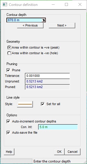
Contour depth |
|
Depth |
The depth of the contour. Note that you can have many contours at the same depth, just like in real life. |
Previous depth |
Change the default depth to be one contour higher (according to the contour interval) |
Next depth |
Change the default depth to be one contour lower |
Geometry |
|
Area is positive/negative |
Select whether to add or subtract the area contained within this contour from the total area corresponding to the depth. This is to account for contours that represent a 'hole' rather than a 'peak'. (Imagine contouring a ring doughnut, contours on the outside would be positive, those one the 'inside' would need to be negative.) In simple maps the area is positive. |
Pruning |
|
Prune |
Use the pruning algorithm to reduce the number of points recorded for each contour. This is particularly useful in auto-tracking mode, or if you like to trace around contours with the mouse button firmly down. While the dialog is open you can toggle this check box and compare the pruned and unpruned data on the map. Note: pruning only works when you first digitise the contour. |
Tolerance |
The severity of the pruning. If you have "Prune" ticked, and change tolerance you can see the effect on the map. |
Unpruned |
The area calculated using the unpruned data. |
Pruned |
The area calculated using the pruned data. This shows you how much you loose (and it will generally be lost) in pruning. |
Line style |
|
Style |
The line style for the current contour. Apply it to all contours with the "Set for all" check box. |
Options |
|
Auto increment |
Add the contour interval to each new contour |
Auto-save |
This auto-saves the srf file |
OK |
The contour is accepted. |
Done |
This button on the main dialog takes you back to the task menu |
You cannot edit contours and add new contours at the same time. Once you've adding, click "Done". The add contour tab goes away and you can edit what you've added.
Click just within the appropriate contour to select it. The nodes (verrtices - where you clicked or where the program assigned a point when auto-tracking) are shown as grey rectangles.
Note: you cannot edit contours and add new contours at the same time. Once you've finished adding, click "Done". The add contour tab goes away and you can edit what you've added.
To move a node, hover over it. The cursor goes to a -||- shape. Click and drag.
To add a mode, hold down the shift key, and then move over the line where you want to add it. It needs to be very close to the line, having added it you an move it as above. The cursor should be a -o- shape.
To delete a node, press the Ctrl key and hover over it. The cursor should be a x shape.
Right clicking on the line brings up the line edit menu:
Delete contour |
Removes it |
Contour definition |
Shows the same dialog as you get at the end of drawing it. Mostly useful to change the depth. |
Contour style |
A dialog allowing you to change the line style of the contour. |
At any time during the editing process you may look at a summary of contours defined so far. By selecting Contours | View Contour table from the menu, you will display a table of contours for the current surface showing depth, pen colour, pen thickness, number of nodes, calculated area under the contour, the area additivity factor (+/-) and a deletion flag. You may alter any of these settings except number of nodes and calculated area.
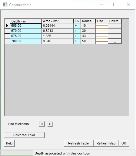
Table |
|
Depth |
Indicates the depth (in feet) of your contour |
Area |
Indicates the area of your contour |
+/- |
+ means the area within the contour is positive (a local peak) or negative (a local depression). |
Nodes |
Indicates the number of nodes used on contour line |
Line |
Choose the line style to draw the contour |
Delete |
Click to delete the contour. |
Line thickness |
Use the two buttons to make the contour lines thinner (<) or thicker (>) |
Universal colour |
Set the line style of all contours to be the same as the current one. |
Buttons |
|
Refresh Table |
Click to refresh table after changes |
Refresh Map |
Click to refresh map after changes |
A block is an areal subdivision of a map. Commonly this can be a licence subdivision (therefore usually with straight line boundaries) but you can make any polygon. Blocks will usually be contiguous (no overlaps) but need not be.
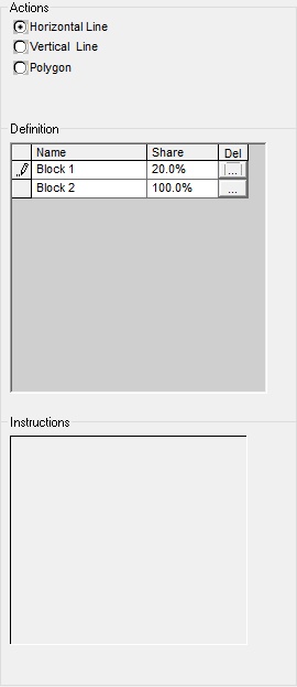
Actions |
|
Horizontal line |
Adds a horizontal boundary across the map. Double click where you want the boundary added. At least two blocks are added (more if the line intersects existing blocks). Name the blocks of the subsequent dialog. |
Horizontal line |
Adds a vertical boundary up the map. Double click where you want the boundary added. At least two blocks are added (more if the line intersects existing blocks). Name the blocks of the subsequent dialog. |
Polygon |
A freehand block. Entered in exactly the same way as a contour (manual mode). |
Definition |
|
Table |
Shows the existing blocks and the percentage ownership in each one. You can also delete the blocks clicking in the "Del" column. |
The on-screen instructions say it all.
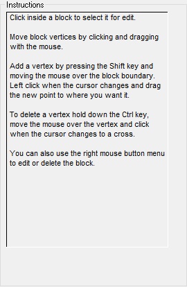
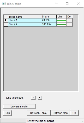
Table |
|
Block name |
Indicates the depth (in feet) of your contour |
Share |
Indicates the your share (ownership) of the block |
Line |
Choose the line style to draw the contour |
Delete |
Click to delete the contour. |
Line thickness |
Use the two buttons to make the contour lines thinner (<) or thicker (>) |
Universal colour |
Set the line style of all contours to be the same as the current one. |
Buttons |
|
Refresh Table |
Click to refresh table after changes |
Refresh Map |
Click to refresh map after changes |
The Area/Depth table (and plot) is a useful tool to check that you have not made any obvious errors when tracing your contours. You can do a similar table and plot for volumes.
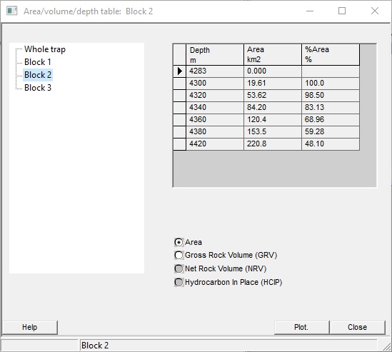
Blocks |
In the left panel you can click on "Whole trap" or any blocks you have defined, to show the relevant numbers in the table on the right. |
Table |
Indicates the area/volumes in each block, and the share of the total |
Show |
|
Area |
Shows the area at each contour |
Gross Rock Volume |
Shows the gross rock volume down to the contour depth |
Net Rock Volume. |
Shows the net rock volume down to the contour depth. Only available when well parameters are entered. |
Hydrocarbon in place |
Shows the hydrocarbon in place down to the contour depth. Only available when well parameters are entered. |
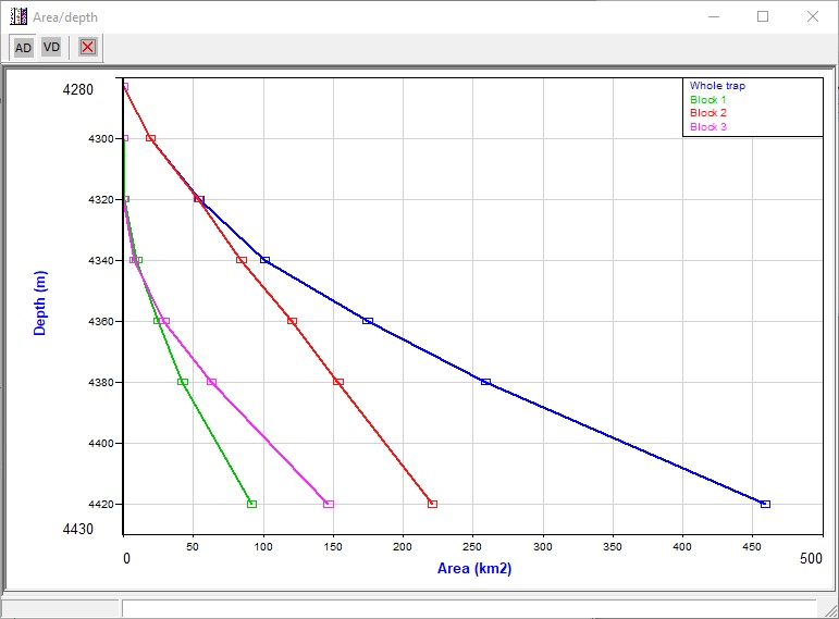
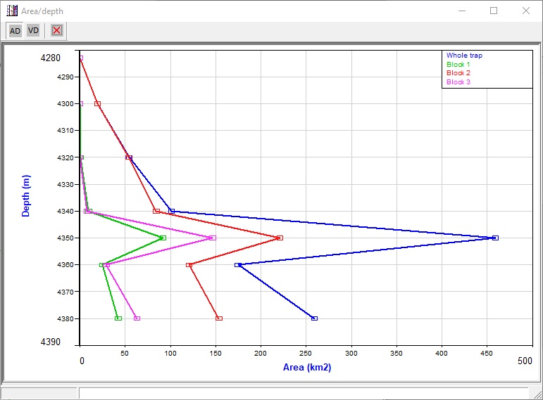
Use the plot button to show are/depth and volume depth plots: these are a good quality control
Example of a good area/depth plot:
Example of an area/depth plot with an obvious mistake:
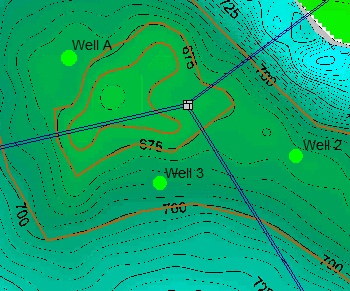
You can show wells on the map. Choose Add mode, and double click at the well location. Enter a well name, well type and status in the next dialog. Assuming the well location is within the span of any existing contours the program will interpolate to find the well top.
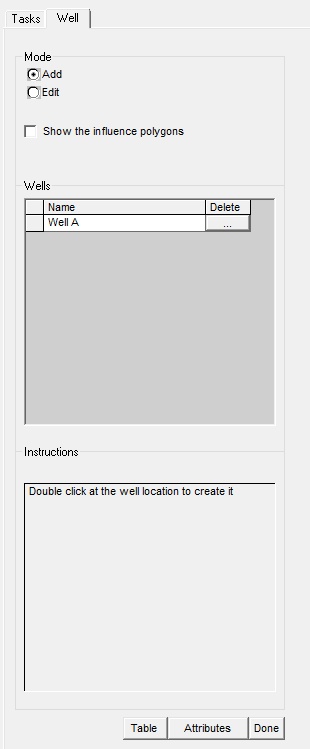
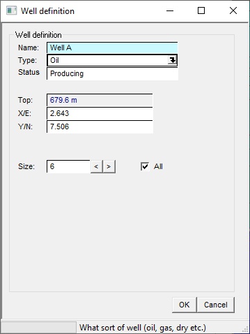
To edit the details later. set Edit mode, right click at the well location and choose "Well definition" from the menu. You can also delete the well from this menu.
Apart from its name. top and location, the well can have any number of user defined attributes. These will commonly be reservoir thickness, net-to-gross (NTG), porosity (PHI) and water saturation (Sw). To set up attributes click the "Attributes" button at the bottom of the Wells dialog,
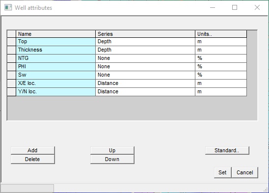
The attributes shown here were created by clicking "Standard". You can add attributes. You should give any numeric attribute a unit and a unit series - use the drop downs lists.
To enter attribute values enter them in the well table:
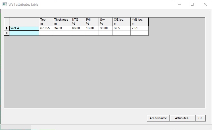
if you have two or more wells defined you can draw "influence polygons" - based purely on distance. Entering the standard attributes will give you estimates of area, gross rock volume, net rock volume and hydrocarbon pore volume for each area. Click Area/volume to see the estimates. This can be a good "first pass" at volumes.
Having created the digitised surface, you will want to save it for future use. Select File | Save or File | Save as to create the .srf file. This is an ASCII file which stores surface identification, name of associated bitmap file, characteristics and co-ordinates of each digitised contour. You must write the map to a surface file if you wish to use it for GRV calculations later.
Select View/Surface File from the menu and you will see the current ASCII surface file.