Calculator

The calculator is a general probability distribution (PDF) manipulation facility. You define PDF's (or load them from existing prospects or consolidations), define an equation and run it. The results of one equation can be used as input to another.

A set of input PDF's and equations/results is a model. You can work with as many models as you like at one time. Models can be saved: the files have the extension ".pdfsim".

When you start, the dialog looks like this:

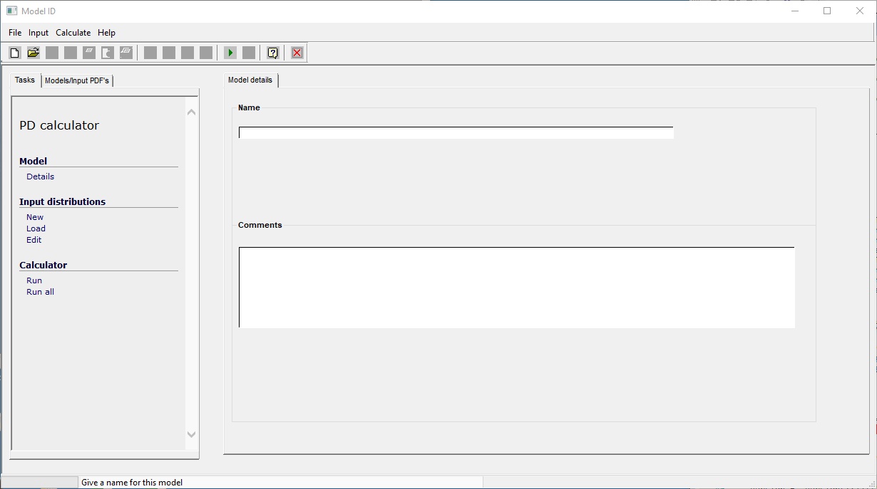
On the left are two tabs: a task menu (all tasks can be run from the window menu and are described below) and a tree list of the models/input PDF's and equations. On the right are are a series of input dialogs and results tables.

The menu items and associated tool bar icons:

File
New model		Start a new model.
Open model		Open an existing model. Model files have the .pdfsim extension.
Save model		Save the current model with its current filename.
Save model as		Save the current model, specifying a new file name.
Print current model		Makes a printout of the current model on the default printer.
Print preview of current model		Makes a print preview of the current model - you can print to any printer from here.
Print all models		Makes a printout of all the models on the default printer.
Print preview (all models)		Makes a print preview of all the models - you can print to any printer from here.
Delete model		Delete the current model.
Exit		Close the calculator window

Input
New variable		Add a new variable.
New equation		Add a new equation.
Add standard variable		Add a standard variable. The tree contains: Prospect input variables (e.g. thickness and porosity) Variables used in estimates of ultimate recovery (e.g. oil EUR per well) Input and output variables from any loaded prospects or consolidations. Variables in the first two categories contain no data, but will have appropriate unit series and unit set. Variables in the last category come complete with the entered or calculated distributions. Click for a typical list of variables when one prospect is loaded.
Delete current variable		Delete the current variable.

Calculate
Run current equation		Run the current equation.
Run all equations		Run all equations.
Iteration control		Allows you to control the iteration procedure. See iteration control below.
Data points
Store data points		Stores the individual data points (input and output values) of each Monte Carlo iteration. Use the "View data points" option to plot them out.
View data points		Plot the stalled data points. See View data points.

Workflow

The usual workflow is

·Start a new model with the icon. Give it a name in the model details dialog.

·Define some input variables, either from scratch or by using predefined or existing PDF's. Input and result distributions in any loaded prospect or consolidation are available. Use the icon to produce a list of all them. Using is highly recommended, because it minimises typing and sets up the unit series correctly.

To review an input, click on its name in the tree on the Models/PDF's tab on the left.

·There's always one (blank) equation when you start a new model. Click on its name in the tree to show the equation dialog. Give it a relevant name and define the equation.

·Run and gasp.

A note on units

One advantage that the calculator has over an ordinary spreadsheet is that it knows something about units. This can also be a hindrance, hence this note.

it works like this: if you define a unit for an input PDF it will convert the values to their SI equivalence. At the end of the calculation it will attempt to convert these SI values into the units of the result.

So it should be the case that if, for example, you multiply an oil density in API units by a volume in millions of barrels and define your results unit as metric tonnes, you should get the answer as a weight in metric tonnes. Confusion may arise if you don't properly define your results unit because their the answers will be in some metric unit which may not have an immediate relationship with the input numbers. On the other hand you can make an equation unhindered by very tiresome conversion factors.

In the calculator (as in REP and LogIC) the units are subdivided into dimensions such as length, volume, density etc.; and further subdivided into "unit series". These unit series are lists of units common to a particular measurement. So, for example, the dimension volume includes unit series named oil volume and gas volume. Within these series you will find the common units (barrels, cubic metres...) for these particular measurements. You will not find cubic inches or acre-feet, even though these are also volumes. You may find the unit series somewhat eclectic, however you will soon find your way through it.

As a provider of oil-field software we do use oilfield unit prefixes: m = thousand and mm = million etc. We apologize unreservedly to our SI-loving cousins. Feel free to blame our late King George III (reigned 1760-1820) who allowed his government to impose tariffs on tea imports into the American colonies. The results were predictable and regrettable; and apparently repeatable.

Units are specified in the unit tree view:

pdf_calc-1

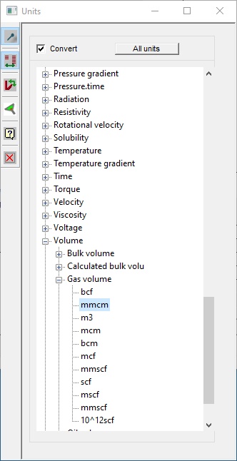
If you have already specified a unit and want to change it, the window shows only the units in the current series. Click the "All units" button to show all the dimensions and unit series.

If you have entered values or are looking at results where the units have been defined and you merely wish to change the unit, the numbers will be converted to the new unit. If you don't wish this to happen un-check the "Convert" box at the top of the window.

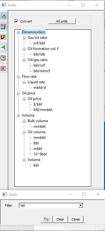
There are occasions (it's quite common actually) when you know the unit but don't know in which series to find it. In this case click the filter button. In the resulting dialog enter the unit and the tree collapses to just those series which contain the unit whole or in part. For example, if you filter on bbl you get:

pdf_calc-1a

Model details

The model details dialog is very simple and consists only of two entries: a model name and comments.

Input Variables

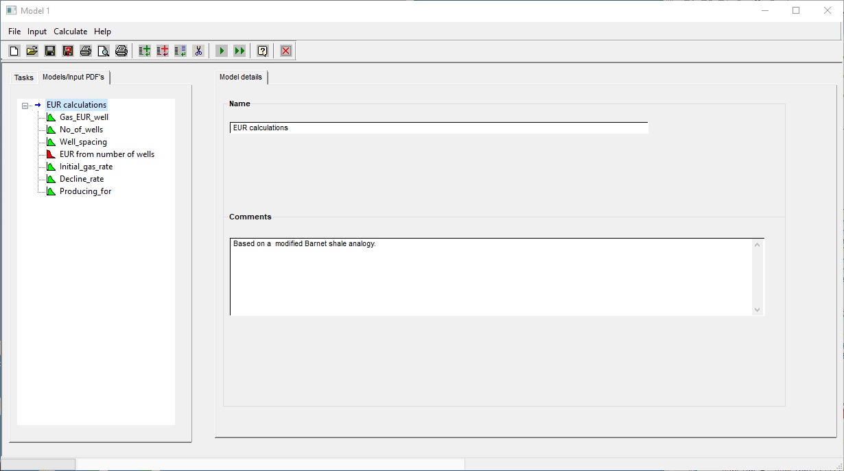
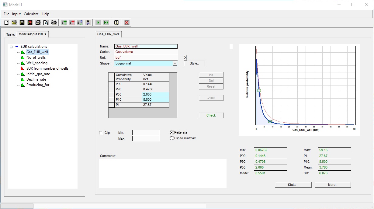
Here is a typical dialog for a model, showing the input variable entry:

ID
Name	The name of the variable. Do not use "/", "+", "-" and "*", all of which will confuse the equation editor because they are valid arithmetic operators. Nor use brackets, for a similar reason. You can use blanks, but they are a nuisance because in the equation you need to put the name in quotes.
Unit	To specify a unit click in the entry and use the drop down tree . This will ensure that not only the unit, but also the unit series is properly recorded
Shape	Choose the probability distribution shape from the drop-down list.
Style	Depending on the shape you have chosen this style button will be enabled or not. Some distributions (and especially normal, lognormal and beta) can be defined in a number of different ways. The style enables you to change the way you enter the distribution. Obviously, the dialogue which comes up will depend on the shape. For example, a lognormal distribution is fully defined by any two points on it. So you have the option to choose which two points you wish to enter.

The table	In the table you enter the values for the distribution. The configuration depends on the shape. In the example shown above the distribution is lognormal and the two points chosen for entry are P50 and P10. Any cell with a blue background need to be filled in. For all distributions probability is in the first column and value in the second. The probability column is usually a cumulative probability, but for user-relative and histogram distributions it is a probability.
The following buttons are applicable and active only for distributions entered as a table: these are histogram, user-cumulative and user-relative.
Ins	Insert a new line in the table.
Del	Deletes the current line in the table.
Reset	Deletes all the lines in the table.
=100	Normalises the relative probabilities to 100%. Used only with histogram distributions.

Check	The check button performs a check on the distribution to confirm that it is properly entered. Note that it will also check against the distribution data limits which you can set (or may be already set) on the dialogue you get when you click the "More.." button below.

Clipping	You can set clipping limits for the distribution.
Clip	Check this box enable clipping of the distribution
Min	The minimum clipping value. If you leave it blank there will be no clip.
Max	The maximum clipping value. If you leave it blank there will be no clip.
Reiterate - Clip to min/max	These radio buttons control what happens during the calculation when a clip is triggered. The default action ("Reiterate") is to reject the current iteration and try again. The effect is therefore to squeeze the entered distribution between the lower and upper clipping limits. The alternative ("clip to min/max") is to limit the chosen variable value to the clip value and carry on. This has the effect of weighting the distribution against the clip. You can see the numerical effect of clipping by looking at the summary statistics below the graph. Without the clip these numbers are shown in black and are for the entered distribution. With clips enabled the numbers are shown in green and are for the clipped distribution.

Comments	It is always good practice to explain what the devil you have done in the comment box.

Summary stats	These are the summary statistics for the entered distribution (in black) or clipped distribution (in green).

More..	Click this button to enter some more details for the distribution. These include: Optional data limits which are used when checking hte distributions. Use clipping to avoid errors when using distributions which exceed the limits Plot limits: by default the variable are plotted using auto-rounded scales. Use these entries to control the minimum plot value, the maximum plot value, or both. A checkbox to disable use of this variable. The most useful effect of this is to stop it being reported out on printouts.

Equation and results

In this dialog you enter the equation to be solved, and enjoy the results

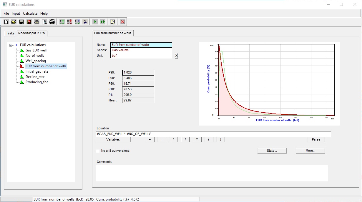
Name	The name of this equation/calculation
Unit	The results unit. See note on units above. To clear the units click the [X] button
P90 etc	These are the results of the calculation
Equation and associated buttons	See below
No unit conversions	Check this box if you don't want the calculator to attempt units conversions.
Comments	Any description of the equation/results you think might be useful.

The equation

The equation is a simple mathematical formula. Enter the right-hand side of the equation only. The equation follows the standard mathematical rules of precedence: exponentiation is done first, then multiplication and division and lastly addition and subtraction. Use brackets in the usual mathematical way to control the order of solution.

Variables are referenced by name, and the name must be preceded by the hash symbol #. If your variable name contains a space (blank character), you must enclose the name in quotation marks.You are recommended to avoid blanks because the quotation marks make the equation harder to read and therefore check.

You should not use mathematical operators in variable names.

Some mathematical functions are available. See the list below.

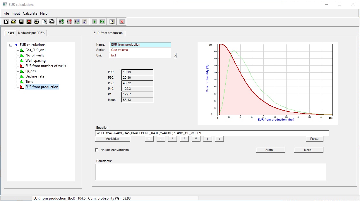
There are also some special functions - see even further below. A special argument has a name followed by a list of argument in brackets, separated by commas. Each argument has a name and a value, separated by '='. The value can be an input variable PDF or a constant value. This example calculates the EUR over 30 years from a shale gas well using hyperbolic decline:

WELLDCA (QI=#Initial_rate, DI=#initial_decline, B=0.5, YRS=30)

Note that some arguments are optional, and if omitted will assume a default value as described below. For example, if you leave out B=0 in the WELLDCA equation it defaults to 0, which is for exponential decline.

Use the buttons described below to build up your equation without tiresome typing.

Buttons

Variables	A tree of the current variables. Click a variable to edit to the equation. It will automatically add the hash symbol and put brackets around names containing blanks.
+ - * / ** ( )	Click to add a mathematical operator or bracket to the equation.
Parse	To check that the equation is written correctly (at least in terms of syntax).

Functions

SQRT	Square root
LOG or LOG10	Logarithm base 10
LN, LOGE	Natural logarithm
CHS	Change sign
EXP	Exponent
ABS	Absolute value
INT	Integer value
NINT	Nearest integer value
SIN, COS, TAN	Trigonometric functions, argument in radians.
ASIN, ACOS, ATAN	Inverse trigonometric functions, result in radians
SIND, COSD, TAND	Trigonometric functions, argument in degrees
ASIND, ACOSD, ATAND	Inverse trigonometric functions, result in degrees

Special Functions (just the one for now)

Note: the argument names can be shortened to just those characters shown in bold

WELLDCA

Calculates EUR (ultimate recovery) from decline curve analysis

WELLDCA arguments

QI	Initial flow rate	Required
DI	Initial decline rate	Required
B	Hyperbolic constant	Optional; The default is 0 (exponential decline)
DLIM	Limiting decline rate	Optional - defaults to 0 (no limiting decline rate)
YEARS or MONTHS	Length of production	Optional - defaults to 600 months (50 years)

Here is an example equation tab for calculating EUR for a shale gas prospect:

Iteration control

This dialog allows you to control the Monte-Carlo iteration process.

pdf_calc-5

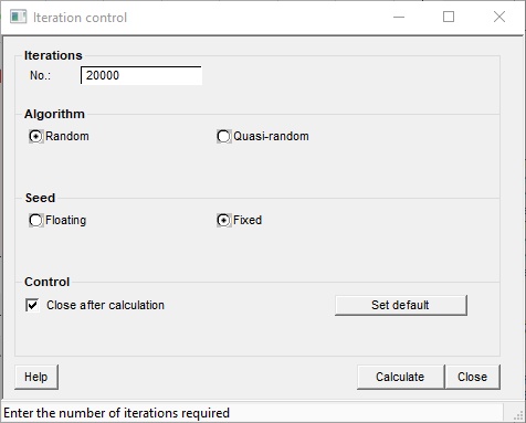
Iterations	The number of iterations in the Monte Carlo simulation. 20,000 is the REP default and gives a stable result in most cases.
Algorithm	Choose random: it's the only one.
Seed	The starting point of the Monte Carlo simulation. A fixed seed starts every simulation with the same value, so you will always get the same result with the same equation. This is useful to prevent the confusion of probabilistic naifs. However, it is not really in the spirit of the method. Purists therefore choose floating.
Close after calculation	Close this dialogue box after you have recalculated by clicking the calculator button below.
Set default	Make these the default values for this model.

Data points

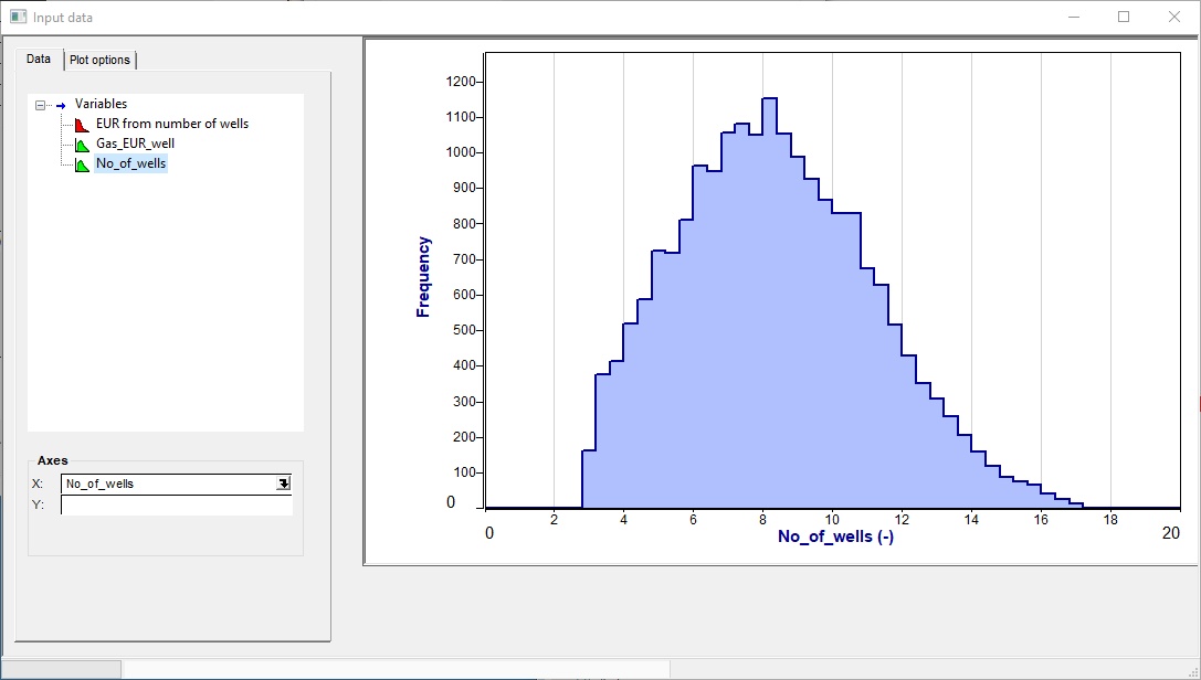
This feature is similar to the data points option in the prospect calculation and consolidation modules of REP. First, you need to run a calculation and store the data. Then choose variables to plot either as a histogram or a cross plot of two variables. The variables can be either input or output probability distributions.

There is obviously a limit to the number of data points that the computer can hold, determined by your machine's resource (memory etc) and the complexity of the equation. If you get no results try reducing the number of iterations in your simulation.

The you don't have a y-axis specified, a histogram will be drawn (see also plot options below):

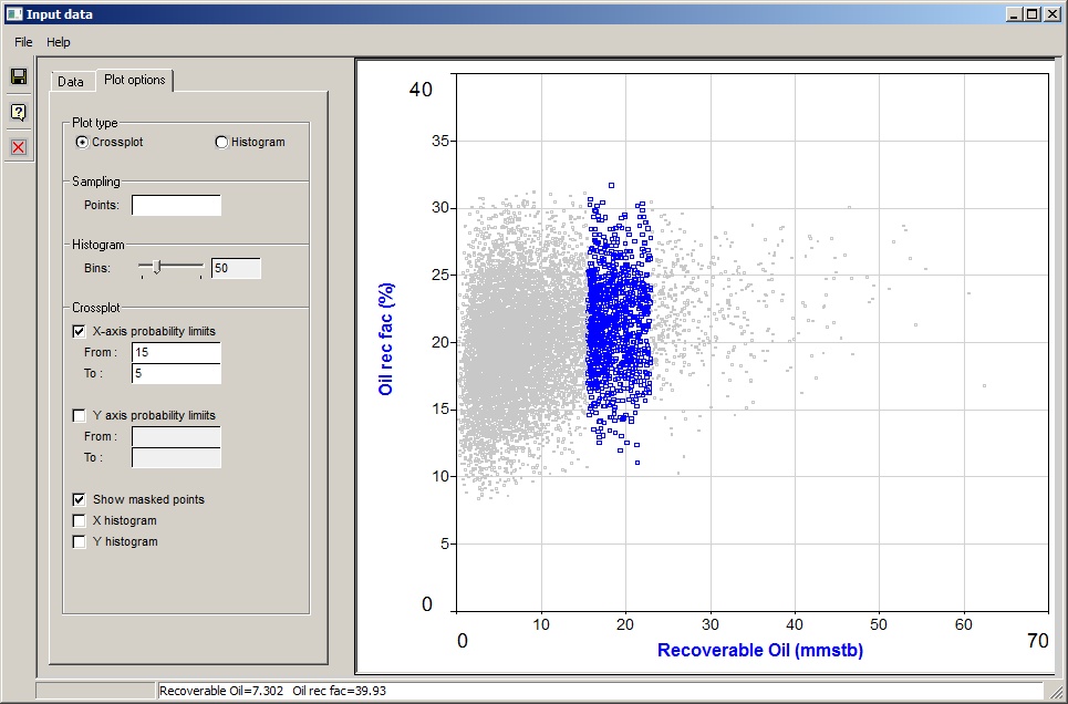
If you specify a y-axis, and "cross-plot" is chosen in the plot options dialog, you will get a cross-plot.

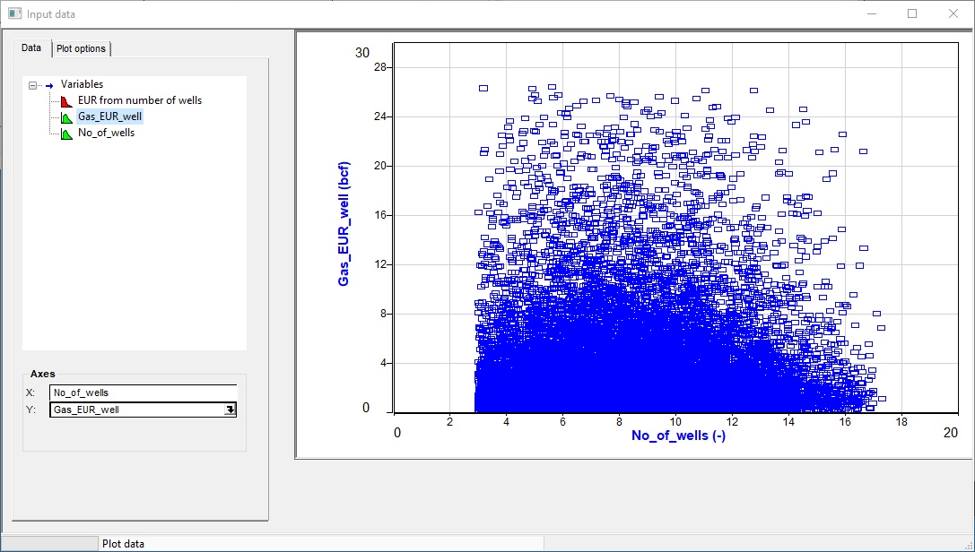
The cross-plots can get a bit dense, since there are as many points as iteration, and the default iterations=20000. Use the sampling option i data point options below to thin them out a bit.

Data point plot options

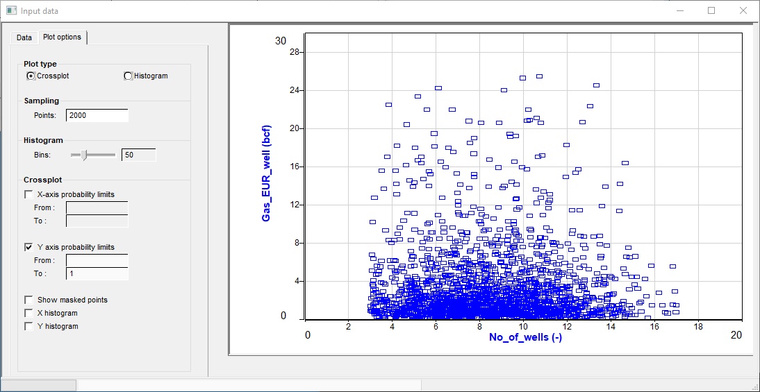
There are some useful controls on how the plots are drawn

pdf_calc-8

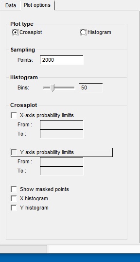
Plot type
Crossplot/histogram	Choose the plot type you want

Sampling
Points	The cross-plots can get a bit dense. Here you can choose to plot a limited number of points.

Histogram
Bins	This is the resolution of the histogram.

Crossplot
X-axis probability limits	You can choose to limit the plotted data to probability ranges in the variable or result. Click to see an example (with masked points being shown) here:
From	The higher probability (P) value - which of course corresponds to a lower value or the variable, since REP uses P100 as a minimum. You can leave it blank, in which case the limit used is 100.
To	The lower P value. You can leave it blank, in which case the limit used is 0
Y-axis probability limits	The same as the x-axis limits, but for the y-axis, obviously.
Show masked points	Check this box to show the points which have been discarded by the probability limit clipping. They are drawn in a discrete grey.
X histogram	Check this box to show a histogram of the x-axis values. This is often obscured by the data points, if you have lots of them. If this happens choose a smaller sampling above.
Y histogram	Ditto.