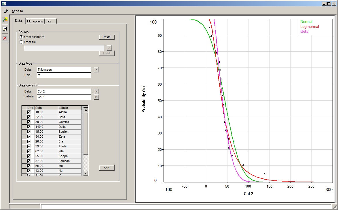
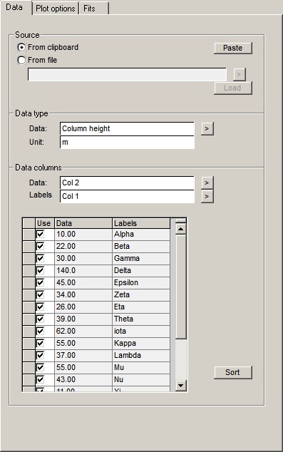
Source

From clipboard

Use this option to load up data from the clipboard. This is the most convenient way to load the data. Use the paste button to load it.

From file

You can also load data directly from an XL or a CSV file. Specify the file name (or browse using the arrow button) and then click load.

The data you are loading should be a table of one or more columns. There must of course be numeric data, but you can also load a column of alphanumeric data which can be displayed on the plots next to the corresponding values.

The software will attempt to recognise column titles and units. It will also attempt to differentiate between numeric and textural data.

Data type

Data

The name of the data you are fitting. If you have come from the probability distribution entry this will be filled in for you. Otherwise choose it from the drop-down tree. If you want to send the fit to the current prospect this entry must be filled in.

Unit

The unit of the data.

Data columns

Data

In this entry specify the column of numeric data, which you wish to fit.

Labels

Here specify a column of data labels. It is not necessary to label the data, but it can be useful.

Table

In the table below the current column of data is shown, also labels if specified. You can remove individual data points by un-checking them in the column titled use.

Sort

You can sort the data by right-clicking a column header. This is useful if you want to remove outliers, though this can also be done by restricting the input to, for example, P95-P5 - see Points selection.

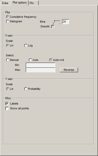
Plot

Cumulative frequency

In a cumulative frequency plot, the x-axis is value and the Y axis is cumulative frequency. Note that the value of the first point does not correspond to P100. Rather, the data are equally spaced in probability with a spacing which corresponds to (n+1) data points.

Histogram

A histogram is a plot in the relative probability domain.

Bins

The number of bins controls the resolution of the histogram. The more bins the spikier it gets.

Smooth

You can optionally smooth the data histogram. Use of this option along with adjustment of the number of bins can e be a useful way of comparing the data with the fits.

X-axis

Scale

The X axis scale can be either linear or logarithmic.

Select

The scale selection can be manual, where you enter the minimum and maximum; auto, where the axis limits are taken from the data; or auto-round, which is similar to auto but the axis end points are attractively rounded down and up.

Y-axis

Scale

Histogram frequencies are always wanted with a linear Y axis scale. But with a cumulative frequency plot the Y axis scale can be on a linear or a probability scale. A probability scale linearises the cumulative frequency curve of a normal distribution. If the x-axis is logarithmic, the probability scale in the y-axis will linearise a lognormal distribution.

Misc

Labels

Check this box to show the data labels next to their plotted positions. This only applies to cumulative frequency plots.

Show all points

If you have used the "Use" column in the data table to deselect some points it can be useful to see where they would have been had they been used in the fit. Check this box to do this.

Note that in probability terms, removing points will alter the value of all the others. So there is a displacement in the y-axis position for the points that are actually used in the fit.

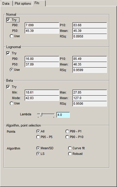
Normal

This box shows the results of a normal fit.

Lognormal

This box shows the results of a lognormal fit.

Beta

This box shows the results of a beta fit. Use the "Lambda" slider to control the lambda parameter of the beta distribution. The default is 4, but

Use

Use this radio button to choose one of the fits to send back to current prospect.

Algorithm, point selection

Points

Point selection is only useful if you have lots of data, and in fact none of the options here will affect the results if you have less than 10 of them. It is a means of controlling extreme values. The data are ranked in order of value and then the chosen range is sent to the fitting algorithm. For example, if you have a dataset of exactly 100 points and choose the 99-P1 option, the first and last data points not be used.

Algorithm

There are two methods (at least) of fitting normal and lognormal distributions. You can calculate the mean and standard deviation and construct the distributions using these two parameters. Alternatively, you can fit the cumulative distribution using least-squares.

In the latter case, you can use standard least-squares (LS) or a robust algorithm, which reduces the influence of outliers.

Note that these options apply only to normal and lognormal distributions. The beta distribution is fitted using a simulated annealing algorithm which does not allow (at least in our implementation) these options. In addition, please note that the beta fit does not always work, especially when there is not very much data to work with.