Calculations

Calculations can be run by clicking Calculate | Calculate from the Consolidations Summary screen. Or just click the Go icon.

There are six other options on the Calculate menu: Outcome distributions, Drilling success envelope, Iteration control, Options, Data Points. and Statistical stability.

Outcome distributions

For each outcome in a consolidation the chance of that outcome, and the P90, P50, P10 and mean volumes are written to a csv file which can be readily loaded up in a spreadsheet (and directly from the program).

You can only run this calculation when all the consolidation inputs are prospects.

Drilling success envelope

This process runs the consolidation with 1, then 2, then 3... etc. entries in the order they are listed in the entry table. The results show the expected volume envelope, GPOS and EPOS as the "drilling program" proceeds. The table gives the results at each step, and these data can be pasted into Excel using ctrl-c (in REP) and paste in excel, in the usual way.

co_dse

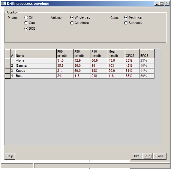
Click the Run button to start the process (which can be quite lengthy, since with n entries the the consolidations is run n times). The Plot button gives a plot like this:

co_dse-2

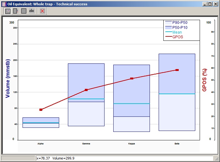
The buttons the top control where the legend is placed (one option is not to have one) and whether you show the names ("abc") in the legend or the meaning of the boxes.

Iteration control

In this screen you can specify whether you wish to use a fixed or floating seed for the random number generator. Computers are unable to generate truly random numbers. Rather, they are given a starting number and from that derive a random(ish) sequence of numbers. But given the same starting point, they generate the same sequence of numbers.

If you use a fixed seed, successive calculations on the same data set and with the same number of iterations will give identical results.

If you specify a floating seed, the program will derive a seed based on the time of day (hours, minutes, seconds and hundredths of seconds) at which you start the calculations. It is most unlikely that successive calculations will have the same starting seed. Using different seeds, the results calculated for the same input data will be different. The amount of difference will depend on the input data and on the number of iterations.

Using a fixed seed is by no means consistent with the spirit of the Monte-Carlo method. But it is sometimes useful to be able to precisely duplicate previous results (if your photocopier has broken down, for instance), or if you are producing management reports. (Some company employees consider that Management gets very confused and bitter if numbers change for no obvious reason, and are liable to go around sacking people indiscriminately. They are, of course, quite wrong to think this. Good managers do not need an excuse.)

You may also specify the number of iterations in a calculation run. Increasing the number of iterations increases the stability of the results, but the calculations take longer. For most data sets, 2000 iterations gives reasonably consistent results. Modern machines are so fast that 20,000 iterations of a prospect only takes a few seconds.

Iteration Control

Iterations
No.	Enter the number of iterations required
Algorithm
Algorithm	Choose the type of algorithm required
Seed
Seed	Choose the type of seed required
Control
Close after calculation	Check to close dialog after calculation
Set Default	Click to set these parameters as default

Calculation options

The only calculation option available is to run a consolidation setting all the underlying prospect risks to 100%.

People really like this option because it gives large numbers. But in a consolidation of undiscovered reserves, the chance of every prospect being a discovery is small, and the more of them there are the smaller it is. The message in the dialog when you choose to use this option is not tongue-in-cheek.

co_calcops

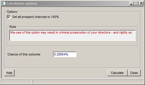
To calculate the "unrisked" results click the calculate button. The chance of the outcome is shown in the dialog.

When you close the dialog, the option is unset; all further calculations are done in the normal way, with the true underlying prospect chances.

You cannot save a file in which the results have been calculated using this option.

Data points

Consolidation data points are very similar to the Data points in prospect calculations, however, rather than comparing two probability distributions, the plots compare one probability distribution for two input prospects prospects.

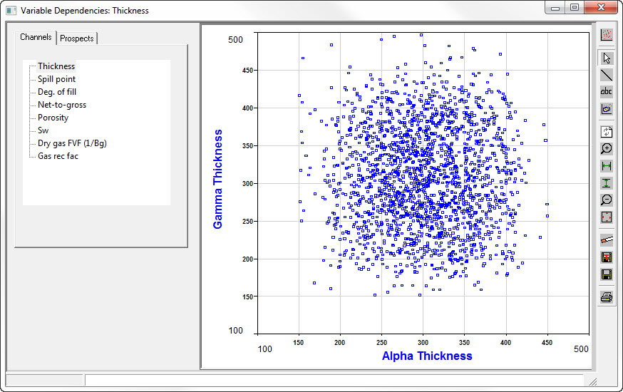
Choose the variable to plot on the first tab labelled "Variables", and the prospects for x- and y-axes on the second tab labelled "Prospects"

	Plot format
	Normal mode
	Line mode
	Text
	Pick points
	Redraw
	Zoom in
	Set X
	Set Y
	Zoom out
	Reset
	Set data filters
	Save plot
	Save plot template
	Print

Storing and saving iteration results

You can store the results of each iteration in a consolidation. Choose the menu item "Calculate | Data points | Store points". Then run a calculation. After this is complete, choose "Calculate | Data points | Save data points". You are prompted for a file name, and the results are written to it. The file is in comma-delimited ASCII format, and can be read into XL directly (in fact, when it has finished writing the file, you are asked whether you wish to view the results, and if you choose "View" REP will launch Excel).

Null results are not written to the output file. The iterations are sorted in order of increasing total BOE, so if you want a case representing the P50, for example. see how many lines there are in the spreadsheet and go to the middle one. Of course it can be readily manipulated in XL anyway.

If your consolidation has consolidation in it, the underlying prospect/field (or dummy prospect) values are shown, but not the intermediate consolidation results.

Note that some consolidations can be large, in terms of both the number of things being consolidated and the number of iterations required. It is possible that the storage space required exceeds the memory available on your machine, in which case this facility will not work. Please let us know this is commonly an issue.

Statistical stability

An occasional question is: how many iterations should I use? This is much more pertinent in a consolidation than in a single volume calculation (unless you are using prospect models) because in a standard prospect case every iteration is a success, with the chance of success calculated separately. In a consolidation, one iteration can have many (or all) input prospects unsuccessful. REP tries to ensure that each phase - oil, gas etc. - of each input prospect has at least the standard number (by default, 20,000) successful cases in the simulation. But even this may not be quite enough if the prospects are very risky, and/or have large uncertainty in terms of P10/P90 range.

In this facility. you run a number of simulations ("passes") with a specified maximum number of iterations with random seed and see the variation of each of the key results: P90, P50, P10 and mean. The variation is also expressed as P90, P50, P10 and mean; this confusion is intentional and is to encourage you not to ask awkward question in future, please.

Here's the dialog, post-calculation:

co_stab-1

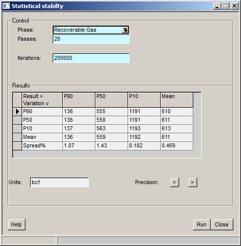
Phase	Choose which phase (GIP, total oil, total gas etc). to display
Passes	The number of full consolidation passes you want to do. Too many of them (especially with lots of iterations) can take a significant amount of time
Iterations	The number of iterations in each simulation pass. Leave this blank to use the the number calculated by REP (based on your default number of iterations if necessary adjusted upwards for input variable chance).
Results	The columns are the consolidation result, the rows the variation in that result.
Spread%	This is (P10-P90)/P50, as a percentage. It's a measure of the uncertainly in the simulation. The more maximum iteration, the less the spread should be.
Precision < >	Click the buttons to decrease of increase the precision with which the results are displayed.
Run	Run the calculation

At the end of each pass, the table updates, and you should see the spreads steadily stabilise (though an "outlier" pass can rock them). As noted above, it can be a slow business, so the "Stop" button in the progress window may stave off terminal tedium. Note that it will only stop after the current pass is completed.