Data points

It can sometimes be interesting to view the actual data that program uses in a calculation. This is particularly the case where you are using dependencies and you want to be completely comfortable with the data that are being used.

To do this you must first run a calculation storing all the data points. From the Calculate menu, choose Data points | Store points. Then run a calculation. Then choose Calculate | Data points | View points. (Actually both these can be done from the latter option).

You can also save the full dataset: the complete set of inputs and outputs for each iteration. You can do this from the main prospect menu ("Calculate | data points | Save points") or when viewing the data points by clicking the save toolbar icon.

Note that there is no theoretical upper limit to the number of iterations, but as you increase the number these plots will get unreasonably solid, and the drawing get slower and slower until your machine starts grinding to a halt. Also, your computer needs to allocate memory to store the data, and there is of course a limit to the amount it can give depending on how well equipped the machine is in this department, and how many variables are in use.

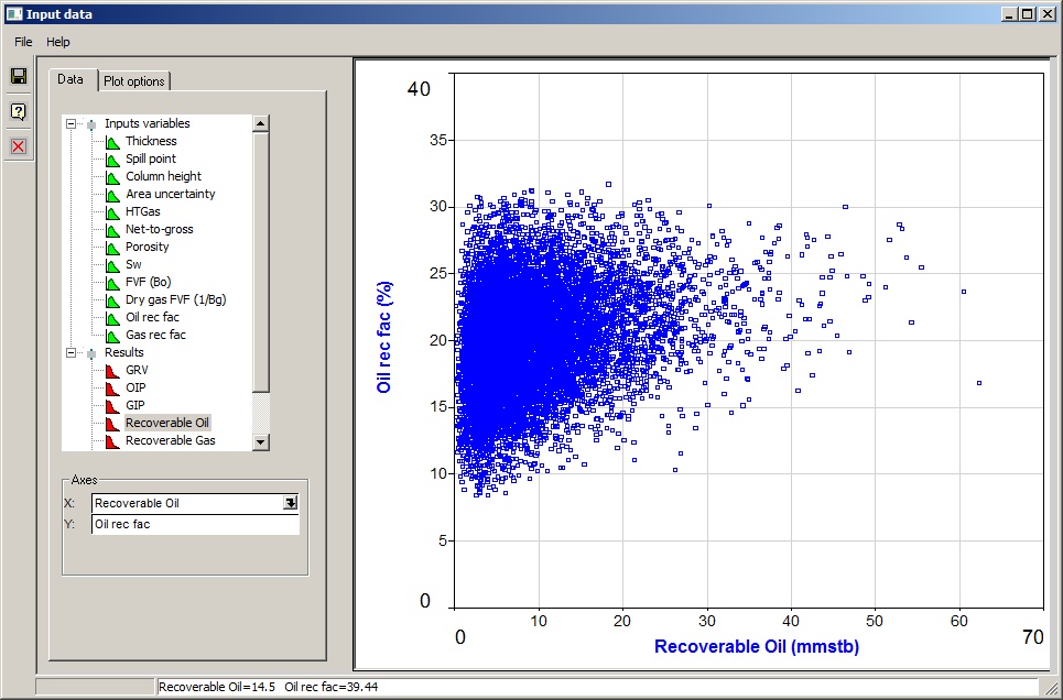
You will then see a dialog similar to that seen below, with nothing plotted yet. On the left is the list of active input variables. There are two ways of viewing the data points: as a crossplot of two variables, or a histogram of one.

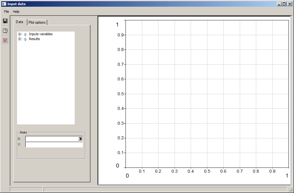
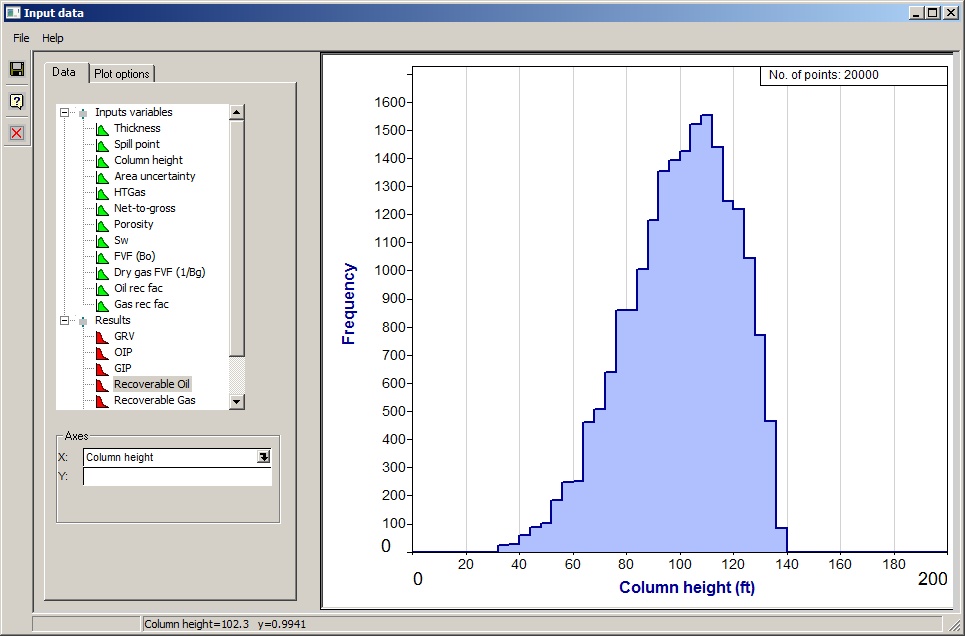
Open the tree branches to see a list of the current input variables and results. Click what you want plotted in the tree. You can also use the drop-downs in the X- and Y-axis entries at the bottom. or drag variables from the tree into the X- and Y-axis entries.

The you don't have a y-axis specified, a histogram will be drawn (see also plot options below):

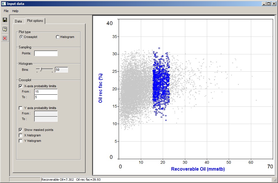
If you specify a y-axis, and "cross-plot" is chosen in the plot options dialog, you will get a cross-plot.

The crossplots can get a bit dense. You could consider reducing the number of iterations to thin them out a bit. There is no theoretical upper limit to the number of iterations, but as you increase the number the plots will get unreasonably solid, and the drawing get slower and slower until your machine starts grinding to a halt.

Plot options

There are some useful controls on how the plots are drawn

pr_data-4

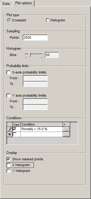
Plot type
Crossplot/histogram	Choose the plot type you want

Sampling
Points	The cross-plots can get a bit dense. Here you can choose to plot a limited number of points.

Histogram
Bins	This is the resolution of the histogram.

Probability limits
X-axis probability limits	You can choose to limit the plotted data to probability ranges in the variable or result. Click to see an example (with masked points being shown) here:
From	The higher probability (P) value - which of course corresponds to a lower value or the variable, since REP uses P100 as a minimum. You can leave it blank, in which case the limit used is 100.
To	The lower P value. You can leave it blank, in which case the limit used is 0
Y-axis probability limits	The same as the x-axis limits, but for the y-axis, obviously.

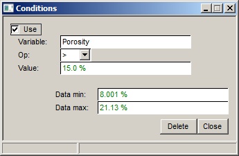
Conditions	Filter the plotted points according to other data values. The conditions are entered in the table. They are logical ANDs
Use	Check the box to use this condition
Condition	The condition
>	Click the button to enter, edit or delete the condition. The dialog is shown here:

Display
Show masked points	Check this box to show the points which have been discarded by the conditions or probability limit clipping. They are drawn in a discrete grey.
X histogram	Check this box to show a histogram of the x-axis values. This is often obscured by the data points, if you have lots of them. If this happens choose a smaller sampling above.
Y histogram	Ditto.