Navigation:  Prospect/Field evaluation > Tools > Reality plots

The central limits theorem is fundamental to statistics and states that if you take a set of independent randomly distributed variables, sample each one and add them up, then the probability distribution of the totals you get by doing this lots of times tends to a normal (bell shaped) distribution.

A corollary is, that if you multiply (rather than add) the input samples, the resulting distribution of products tends to a log-normal shape.

In the context of prospect evaluation, the theorem can be restated: where the fundamental processes controlling the amount of hydrocarbon reserve are multiplicative, the resulting reserve probability distribution should approach a log-normal shape.

So when REP multiplies GRV, net-to-gross, porosity, hydrocarbon saturation etc., the answer usually looks log-normal - and you can see this from any REP calculation.

Many of the standard REP inputs are themselves products of more fundamental processes. For example, GRV is the product of area and thickness (sort of), and reservoir thickness may be the product of rate of deposition and how long the deposition went on for.

Some authors insist that all input parameters have multiplicative origins and that as a result you should only use log-normal distributions as input. There are practical as well as theoretical difficulties with this position.

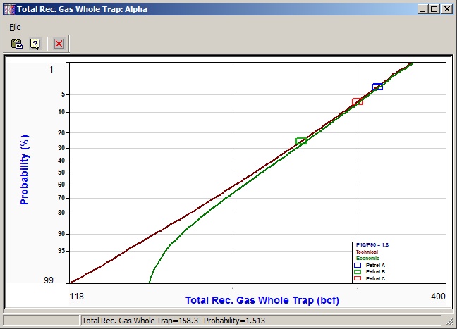
But no one disputes the central limits theorem and so the reserves distribution from a REP prospect/field calculation should be approximately log-normal. In a reality plot, the cumulative reserves distribution is plotted with the reserves axis on a logarithmic scale and the probability axis on a normal probability scale. If the resulting graph shows a straight line, then the distribution is log-normal.

If it is not log-normal, then you should consider arming yourself with a decent explanation of why.

Sometimes, the middle probability values are high (in reserve terms) compared to a straight line drawn between the endpoints (the P95 and P5 values, say). This is exactly the situation that log-normal fanatics like to see. They will rub their hands together with gleeful anticipation and then reach for their instruments of torture. They will argue that you have boosted the middle values (upon which most economic evaluation rely) in order to get your prospect approved and drilled. Or they will say that you have not considered in sufficient detail the upside, thereby undervaluing the prospect and condemning your company to endless mediocrity.

All this can be avoided by looking at the reality plot and taking evasive action.

[Note: Most practitioners use the technical and ignore the economic.]

The plot legend also shows the P10/P90 ratio. This is considered to be a very diagnostic number. It is of course a measure of the uncertainty in volume, and should therefore reflect the maturity of the prospect. Here are some guidelines:

Development:  1.5 - 2

Appraisal: 2 � 5

Near field step-out: 4 � 10

Green field: 5 - 20

Frontier: 10 � 50+

Not everyone is not convinced that these numbers are useful, and some recent papers have argued the case against even more strongly than this.

 

You can show deterministic estimates on the plot. These are presumably calculated outside of REP - by a static or dynamic model, for example, or by third parties. Plotting them up on the reality plot can be a good sense check, of both sets of numbers. Enter the deterministic numbers in menu option "File | Other data | Deterministic estimates"