Prospect Models

Sometimes, you have different interpretations of data, only one of which may be correct. In prospect calculations, different interpretations may relate to different hydrocarbons being present (oil, gas), different trapping mechanisms (structural, stratigraphic) or different depletion strategies (water injection, primary recovery). Creating different models is a much sounder strategy than smearing distributions to account for different interpretations.

Each model is assigned a relative probability of occurrence - relative, that is, to all the other models. The sum of all the model probabilities (chances) must be 100%.

In earlier versions of REP (pre v5.10) combining models was done using 'consolidation of mutually exclusive events'. This option still exists, but using this models facility is much preferred.

File
Add a new model		Click to add a new model
Import a model		Click to import a model from a REP .ppr file
Delete model		Click to delete the selected model
Exit		Click to exit Models dialog

Edit
Move Up		Move selected model up
Move Down		Move selected model down
Demote		Make the selected model a "child" of the model above it in the table. This means that the selected model is only possible if its parent is "true".
Promote		Remove the child status of the selected model
Show		Click to show the risk decision tree

Chances
Use fixed chance		The model relative chances are fixed.
Target final GPOS		Makes the final GPOS the model GPOS for simple dependent model cases. In other cases this option is greyed out. See Dependent models: GPOS and model chance below.
Use relative chance distributions		The relative chances are themselves probability distributions. This applies to all model branches. See below for an example where this could be useful. To enter a chance distribution, click the drop arrow at the right of the model chance entry in the table.
Add all chances and normalise		Each model must have a chance distribution. On every iteration, the distributions are randomly sampled, the chances normalised an one model chosen at random. (In other words, the chance distributions are possibilities rather tha probabilities.)
For two models, use only the first distribution		Where a branch of the model tree has two (and only two) model outcomes, you need only enter one chance distribution - which must be for the first model.
Warning entry		This warning box tells you when either the chances are not normalised (for fixed chances) or when some chance distributions need to be entered (when using relative chance distributions).
Normalise		Click to normalise chances so they add up to 100% at each branch.

Defining Models

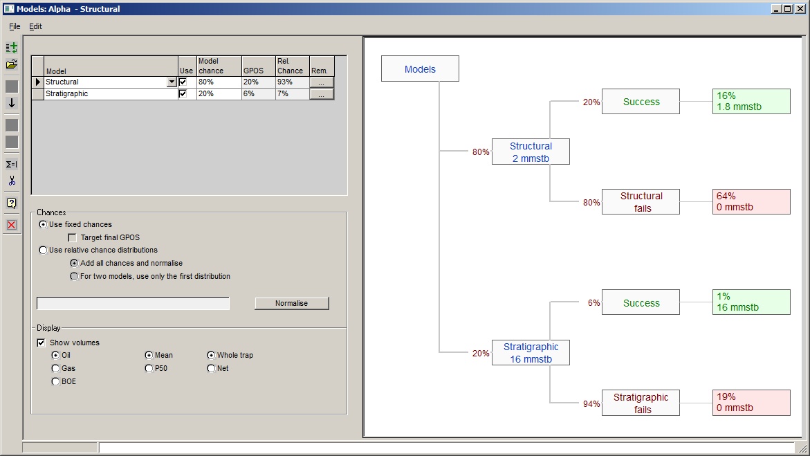
When you define any new prospect, one model is created. To make another, go to Parameters | Models.

The window that appears shows the current models and the relative chance of each one. If there is only one model the relative chance should be 100%, of course. To add a new model, click the [New] or the [Import] button.

Add Model

·[New] creates a new model by making a copy of the existing model. The existing model is indicated in the list of models with the > symbol to the left of its name. Give the new model a relevant name and rename the old one if necessary.

·[Import] will read an existing prospect file. Note that some prospect specific information (prospect ID mostly) will not be imported. These data are discarded in favour of the current prospect's details.

To delete a model, click the [Delete] button. From the point of view of the calculations, setting its relative chance to zero will have the same effect.

The [Normalise] button alters the relative chances so that they add up to 100%*.

[*Note: The program will do this anyway at the beginning of any calculation.]

Viewing Models

In the prospect list on the left of the summary screen all the current prospects are shown. Prospects with more than one model show the models as branches in the prospect list. The data shown in the summary screen reflects that part of the prospect which is highlighted in the tree list.

If you have one of the models highlighted (or you click on it to highlight it), the summary screen data shows the results of that model only.

If you have the prospect name highlighted, the summary screen data shows the results of the full prospect calculation (all the models combined).

If some or all of your models have layers, these are shown as further branches in the tree and if you highlight one of the layers the layer data will be shown in the summary screen.

Variable chances

There are some circumstances when using variable chances can be useful. One such is where the two models represent different facies. You may have some statistics about the likely proportion of facies, and the chance distribution can reflect this. In this case the two models represent the end members, and the final result is the answer you want.

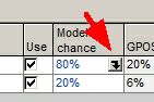
When using chance distributions, the model chances shown in the tree are the means of the distributions, normalised across each branch.

Results

It is important to realize that different models can (and often will) have different geological risks as well as different relative chances.

For example, you might consider that a given prospect has a 30% chance of being a structural trap and a 70% chance of being a stratigraphic trap. You might also reckon that if the mechanism is structural then the chance of a seal is 90% but if the mechanism is stratigraphic then the chance of a seal is only 60%. When REP combines these 2 models it calculates the seal chance as the weighted average of the two models:

Final = (COSseal x model chance)|model1 + (COSseal x model chance)|model2

= (0.9 x 0.3) + (0.6 x 0.7)

= 0.27 + 0.42

= 0.69

All the geological risk factors are combined in this way and they are multiplied through to give a geological chance of success (GPOS) for the combined prospect.

The economic chance of success EPOS is only relevant to the combined prospect results since economic cut-offs are only applied at a prospect level. In other words, individual models do not have an EPOS, only a GPOS.

If you have two models, one an oil case and the other a gas case, do not forget to define economic cut-offs for both oil and gas (or neither). If, for example, you define an oil cut-off but not a gas cut-off then every gas case realisation will fail the cut-off criterion because it has insufficient oil.

[Note: Remember that to pass the economic hurdles, either the gas volume must be greater than the gas cut-off or the oil volume must be greater then the oil cut-off]

It should now be clear that when combining models in a prospect calculation you will have a GPOS, which is the combination of the model GPOS's; and an EPOS, which is the chance of an economic success.

Both GPOS and EPOS tell of the chance of success of the prospect, they say nothing about models. It can get confusing when you are looking at recoverable oil results for a prospect which could be either oil or gas. GPOS and EPOS describe the chance of success of finding either oil or gas. But the oil numbers refer only to what you discover if you discover oil. REP calculates a "Phase Chance", which is the chance of a particular phase (hydrocarbon type) being discovered. Mostly, REP reports phase chance as a relative probability. For example, in a prospect with a GPOS of 18% and an oil phase chance of 60%, the chance of discovering oil is:

Chance of oil = GPOS x Phase chance

= 0.18 x 0.6

= 0.108

Dependent models: GPOS and model chance

Where you have dependent models (one model depends on the success of another) the GPOS vs. model risk becomes a bit complicated.

There are two ways to look at the chance of success of a particular model.

oThe chance that the model will contain oil or gas, should the model be realised.

oThe chance that should oil and gas gas be discovered, this model is the one realised.

Th first is the way that you should usually think about it, because (in a complicated system) the GPOS describes the relative occurrence of the two model outcomes: success and failure. But in simple dependent systems that's not always the way that you do think about it.

Consider the common case of a prospect with 4 way dip closure, but possibly a deeper fault seal. There are two models - 4-way closure and deeper fault seal. If the deeper fault seal works, the 4-way closure must also work. If the 4-way doesn't, the deeper seal cannot. So the fault seal is dependent on the 4-way. Here's the tree view:

pr_models7

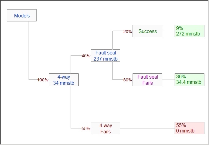
There are three possible outcomes (bottom to top in the picture):

oThe 4 way dip closure is dry - no hydrocarbon at all

oThe 4-way works, but the closure against the fault doesn't

oThe fault seal works, so so does the 4-way.

Now consider the GPOS's. As entered by the user (for we are optimists, at Logicom E&P) the 4-way is 45%, and the fault seal 20%. There is no confusion with 4 way, and this is the controlling chance of success for the prospect. But the 20% GPOS for the fault seal assumes that the 4-way works. From the outcome boxes, you can see that there is overall only a 9% chance (=0.45 x 0.2) that the fault seal will work. A bit different to the 20% the user might have expected.

The purpose of the check box labelled "Target final GPOS" is to modify the effective GPOS of the dependent model so that the final chance of the fault seal working is 20%:

pr_models8

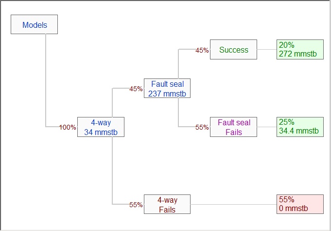
The top box on the right now shows 20%, which is the original GPOS of the fault seal model. The 4-way works in the top two boxes, the sum of which is 45%, as entered.