Prospect/Fields summary

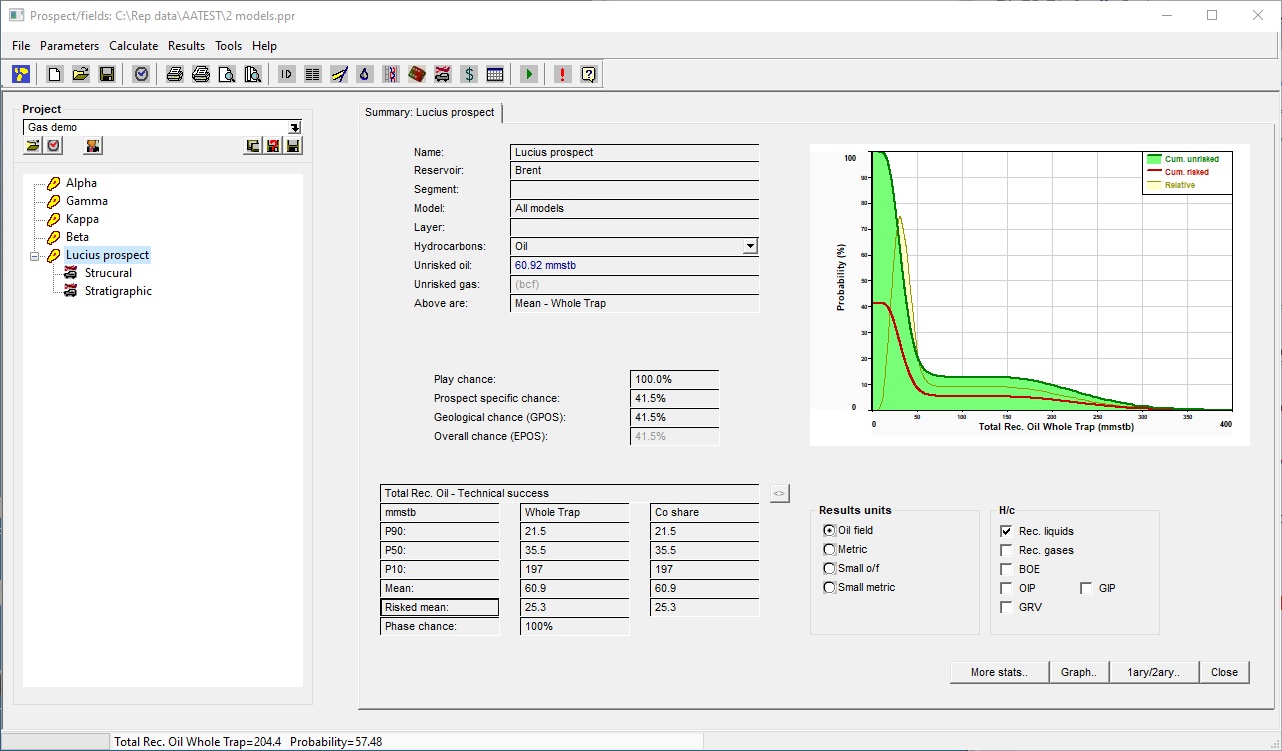
The prospect summary screen controls all of the prospect entry, calculation and results tasks.

On the left of the window there is a list of all the prospects currently active. Since each prospect or field can have multiple segments*, each segment multiple models and each model multiple layers, there is a "tree" hierarchy. You can click on any branch to make this prospect/segment/model/layer active. You can also remove prospects from the list by right clicking on the prospect and selecting [Remove].

[*Note: depending on program version, segments may not be activated.]

To the right is a summary of the active prospect/segment/model/layer is shown. See Results Summary, below.

At the top of the window is the menu bar from which all actions are initiated. Common actions also have buttons in the tool bar. See 'Prospect/Fields Menu' for more information.

By default, the results plot has automatic scaling. If you right-click in the plot you can set the scales - see below.

Project
Project	The current project: if no project has been opened it shows "Default" Click the drop-down arrow for the project menu. Here you will also find out what those buttons do, and also how to organise prospects and consolidations within a project.

Prospect summary
Results units	Select desired unit for results output
H/c	Toggle between hydrocarbon types
More stats..	Click for more detail on the results distribution
Graph..	Show summary graph in new window. You can also double click in the graph area.
1ary/2ary..	Shows the split between primary (matrix) and secondary (fracture) volumes in the case of a dual porosity system.
Close	Close selected prospect summary

Results Summary

When you first read a file, the summary results are taken from the file. When you change a parameter and run a calculation, the screen is updated with the new results.

If you have more than one prospect active, you can click the prospect (or layer/model/segment) to see its particular results.

The summary shows the ID of the Prospect (and the current segment*, model and layer) at the top left of the screen. Below are shown the defined hydrocarbons, and the unrisked mean quantity of total recoverable oil (liquids) and gas. These can be either whole trap or net (company share), depending on the entry in the Installation Options.

[*Note: depending on program version, segments may not be activated.]

Then comes a summary of the chances of success - "Play", "Prospect specific", "Geological Chance of Success (GPOS)" and "Economic Chance of Success (EPOS)". If there is no economic cut-off defined, the GPOS is equal to the EPOS.

Below the chances, the key numbers are shown. The P90, P50, P10 and Mean figures, both whole trap and net, refer to the success case - i.e. the outcome if hydrocarbons are discovered. The risked mean is the mean multiplied by the technical chance of success (GPOS).

Where there is no economic cut-off, and GPOS = EPOS, all these numbers are shown in black.

Where there is an economic cut-off, there are two possible success cases: technical and economic. You can look at either and switch between the two by toggling the [<>] button. The technical success case numbers are shown in red, and the economic success case is shown in green.

Note that the economic success case mean is always equal to or higher than the technical success case mean, and the displayed risked mean is always the technical success mean multiplied by the GPOS, i.e. the risked mean does not change.

The mean is either the arithmetic mean or Swanson's mean (in which case it is shown as "Mean Mz"). You can choose which to show in the Installation Options. Because of the way REP clips its skewed distributions there is normally not much difference between the arithmetic mean and Swanson's number.

To the right of the summary is the results graph. This shows the probability against the reserve. See 'Understanding the Results' for a discussion of what the curves are.

Below the summary numbers are some buttons:

[More stats..] gives slightly more detail on the results distribution (including both the arithmetic mean and Swanson's mean)

[Graph..] shows the summary graph in a standalone window. There are three reasons you might wish to do this.

1. You can make it big, so that even blind management can see it.

2. You can paste it onto the Windows pasteboard (using <CTRL+ALT+PRNTScreen>) and then copy it from there into any Windows program, or print it using the window print option.

3. You can save the data in the graph as a comma-delimited file, and read the data into XL. Some people find this useful. Use the window File | Save as option.

[1ary/2ary..]

[Close] closes the selected summary.

To the right of the summary screen, below the graph, are four radio buttons, which enable you to change the output units, and five check-boxes which enable you to toggle between hydrocarbon types.

Here is a description of the toolbar icons

	Open consolidation dialog (or bring it to the front if it's already open)
	Click to start a new prospect
	Click to open an existing prospect
	Click to save prospects
	Opens the database module.
	Click to toggle evaluations
	Click to print summary
	Click to preview summary
	Click to open ID dialog
	Click to open Description dialog
	Click to open GRV dialog
	Click to open Hydrocarbons dialog
	Click to open the sorbed gas dialog (CBM and shale gas prospects only).
	Click to open Petrophysics dialog
	Click to open risking dialog
	Click to open Models dialog
	Click to open Economic Criteria dialog
	Click to open Summary dialog
	Click to calculate
	Show any current information or error messages
	Click to open Help