Prospect/fields Menu |
  
|
Prospect/fields Menu |
|
The menu toolbar above the Prospect/Fields summary screen allows you to navigate through the module.
![]()
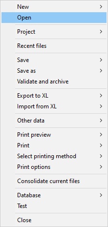
The Prospect/Field menu has these main options:
·File: Opening, saving, printing, etc.
·Parameters: Input of all parameters required for a prospect calculation.
·Calculate: Full calculation, single point calculate, set calculation parameters (iterations).
·Results: Choose which hydrocarbon type (recoverable oil, gas-in-place, etc.) to view.
·Tools: Diagnostic plots, sensitivities, production profiles, etc.
·Help: Access to the help pages.
New | Prospect
This starts a new prospect. To enter parameters, use Parameters | All, as outlined below, in Parameters.
Starting a new prospect can also be achieved by clicking on the ![]() icon.
icon.
This opens the New Evaluation dialog. See 'Prospect Evaluation' for more information.
To reveal or hide evaluations, click on the ![]() icon.
icon.
This opens an existing prospect. The standard Windows "File open" dialogue is displayed. You can choose one or more prospect files to open, using the standard Windows procedure.
Opening an existing prospect can also be achieved by clicking on the ![]() icon.
icon.
This allows you to group together prospects and consolidations. See 'Projects' for more information.
In the sub-menu the most recent prospect files (up to 20) are shown. Click on one of them to load the file. You can load all of the recent files at once by choosing "Load all recent". You can also clear the recent files list by choosing "Clear all recent".
Under the "File | Save" menu option you have the option to save all loaded files or just the current one. You can also load it/them into the prospect database.
Saving the current prospects can also be done by clicking on the ![]() icon.
icon.
Under the "File Save as" menu item your can:
Save the prospect with a new file name
Save the prospect in ASCII format (an option for geeks)
Save as a new prospect. This produces this dialog:
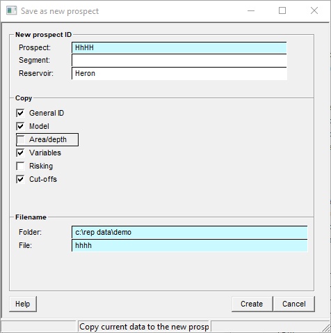
Choose a new name and those elements of the existing prospect that you wish to copy over.
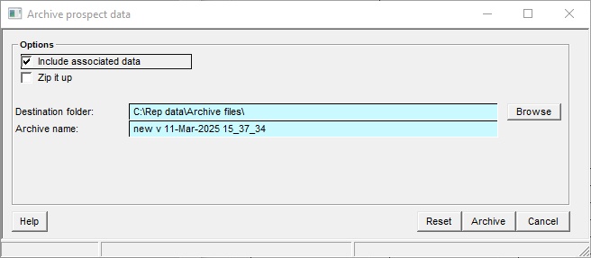
This will check that mandatory entries are completed (but will not check their integrity, of course) and then make a time-stamped copy in the archive folder (or elsewhere if you wish).
This has several sub-options:
"XL prospect file" writes prospect data into an XL spreadsheet. See 'Exporting Data to XL Spreadsheets' and 'Data Export Templates'.
"XL summary file" writes prospect summary into an XL spreadsheet, possibly a prospect inventory. See 'Exporting Data to XL Spreadsheets' and 'Data Export Templates'.
"Copy to clipboard" copies key numbers for the current hydrocarbon phase to the Windows clipboard. From there they can be pasted into Word, XL, etc. for reformatting and presentation.
There are 2 sub-options:
![]()
New prospect is appropriate when you have a spreadsheet with input data from an outside source. See Import from XL.
From XL multi-tabbed file is used when you've exported data from REP, and have made changes in the exported spreadsheet. The changes can then be re-imported. The assumption is that (a) the prospect already exists in REP and (b) the exported XL spreadsheet has the prospect (ppr) file name written somewhere, so that the link can be easily made.
It can be useful to list non-REP files (spreadsheets, reports, maps etc.) that are related to a prospect as a simple document list. See 'Associated Files' for more information.
Deterministic estimates: 3rd party results: click here for details
These options produce the hard copy output. "Print" sends it straight to the printer. Printing is via the Windows system, so any printer accessible to your computer can be used. "Print preview" draws it on the screen, you can send it to the printer from the preview window. "Windows metafile" writes the printed sheets to .emf (metafile format) or .bmp (bitmap format). Both are readily imported into other windows programs, including word, XL etc. See 'Printing' for more information.
[Note: With all the printing options, you can choose to print the "summary pages" (the key input and results, by hydrocarbon type), the "full" output (about 5 pages, depending on the hydrocarbons present) or a "selection" of pages.]
Printing a hard copy output can also be achieved by clicking on the ![]() icon.
icon.
Loading a print preview can also be achieved by clicking on the ![]() icon.
icon.
Select "All options" and a screen will appear in which you can choose to make your output in CGM format. CGM is a common graphics format which can be read by many oil-field software packages, including the ZEH plotting system. You can also choose not to show economic criteria on output sheets. Economic criteria is often rather sensitive data, so this is a useful option if you are giving your results to partners.
Select this to reveal a standard printer dialogue box in which you can set page size and other printing parameters. Do not trouble to set the page to landscape.
All the current prospect entries are loaded into a new consolidation. The consolidation is run and the results shown in the consolidation summary screen.
From the parameters menu all the input data can be entered and edited:
If you are starting from new, this option runs through, step-by-step, all the other parameter menu items allowing you to enter the data in a structured manner.
A simple dialog in which the relevant resource type can be chosen. See 'Resource Type' for more information.
A simple dialog in which you can chose the default unit for input: oil field or metric. See 'Unit Type' for more information.
Note: You can override the default for any input parameter.
This dialog allows you to enter the prospect name, location, setting and other general descriptive data. See 'Prospect Identification' for more information.
The Identification dialog can also be opened by clicking on the ![]() icon.
icon.
This dialog allows the user to summarise the key geological features of the prospect. See 'Prospect Description' for more information.
The Geological Description dialog can also be opened by clicking on the ![]() icon.
icon.
Here, all the parameters controlling the GRV model and associated data can be entered. See 'Gross Rock Volume' for more information.
The Gross Rock Volume dialog can also be opened by clicking on the ![]() icon.
icon.
A dialog in which the hydrocarbons that either are, or you hope are, present in the prospect can be selected. See 'Hydrocarbons' for more information.
The Hydrocarbons dialog can also be opened by clicking on the ![]() icon.
icon.
This is a dialog in which the reservoir petrophysical parameters are entered as probability distributions. See 'Petrophysics' for more information.
The NTG/Porosity/SW dialog can also be opened by clicking on the ![]() icon.
icon.
This is a dialog in which the expected relationship between recoverable and in-place volumes are entered as probability distributions. See 'Recovery Factors' for more information.
Here, relationships (if any) between the input variables can be described. See 'Variable Dependencies' for more information.
Use this dialog to evaluate the chances of success. See 'Prospect Risking' for more information.
The Risking dialog can also be opened by clicking on the ![]() icon.
icon.
This option produces a summary of all the risks in all the loaded prospects. See Risk table.
This dialog is used to enter the minimum values of oil and/or gas for the prospect to be economic. See 'Economic Cut-offs' for more information.
The Economic Cutoffs dialog can also be opened by clicking on the ![]() icon.
icon.
This is a useful facility which allows you to view and edit all the input parameters from one place. See 'Input Data Summary' for more information.
The Input Data Summary can also be opened by clicking on the ![]() icon.
icon.
Use this facility to add (or remove) alternative models for your prospect and their respective probabilities. See 'Prospect Models' for more information.
The Models facility can also be opened by clicking on the ![]()
This dialog allows you to enter reservoir layers with separate properties. See 'Prospect Layers' for more information.
This facility runs a calculation on the current prospect file or you can chose to "Calculate All" open prospects.
The Calculate facility can also be run by clicking on the ![]() icon.
icon.
This option enables you to run a "single point" or deterministic calculation, i.e. solve the volumetrics equation with a single value for each parameter. See 'Deterministic Calculations' for more information.
Here are some further options controlling the way calculation is made See 'Calculation options' for more information.
Data Points
See 'Data Points' for more information.
The menu options are a list of all the relevant hydrocarbon types produced or present in the current prospect. Choose one of them to see the results for that hydrocarbon type in the summary window. You can also show the area/depth plot (if there is one), GRV and in-place volumes. See 'Understanding the Results' for more information.
From the tools menu you can produce some useful sensitivity and QC plots:
This is a spider graph that shows the influence on the results of all the input parameters. See 'Sensitivity Plots' for more information.
This is a simpler version of the sensitivity plot where all the parameters are ranked in terms of the overall influence they have on the result. See 'Sensitivity Plots' for more information.
This is a useful QC. See 'Reality Plots' for more information.
This allows you to create a 'quick and dirty' production forecast based on one or more reserve levels and quickly export it to XL. See 'Production Profiles' for more information.
This allows you to see the influence of any economic cut-offs on the results. See 'Economic Cut-offs' for more information.
This allows you to create scenarios, which correspond to each probability case. See 'Realizations' for more information.
This tool allows you to compare variable probability distributions in a group of prospects. See 'Prospect Input Data Plots' for more information.
Help refers to the general REP help. Custom Help are help pages written for a specific site, and not available to other REP users.
REP Help can also be accessed by clicking on the ![]() icon.
icon.