Entering probability distributions |
  
|
Entering probability distributions |
|
This section is in four parts:
What is a Probability Distribution?
Probability Distribution Shapes
You may also want to refer to the section 'Input Variables'.
Since almost all of the numbers used by the program in its calculations are in the form of probability distributions, it is important to understand them. Here is the standard dialog for entering all the probability distributions in REP.
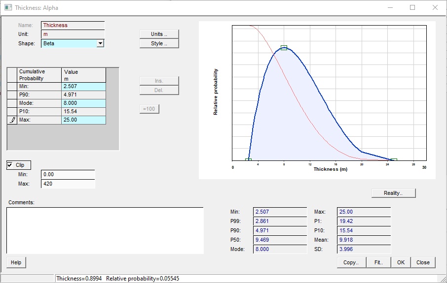
Name |
The name of variable |
Unit |
The unit of variable |
Shape |
The shape of the probability distribution (normal, log-normal, beta, triangular etc.) |
Units |
Click to set the unit for the variable. On the pop-up dialog, note the "convert values" check box. If you have entered values in the wrong unit, uncheck the box and set the new (correct) unit). The values remain unchanged, just the unit is set. If the box is checked, any entered values are converted from the old unit to the new one. |
Style |
Click to change the entry method for normal, log-normal, beta and triangular shapes. Each has its own options - see Styles below |
Ins. |
Click to enter a new line in the table: this is used only for histogram distributions. |
Del. |
Click to delete selected line in the table: this is used only for histogram distributions. |
=100 |
Click to normalise the sum of probabilities to 100%: used only in histogram distributions. |
Reality.. |
Click to draw a reality plot of the probability distribution. A reality plot shows the probability distribution with the variable value on the x-axis using a log scale and the probability on the y-axis using a probability scale. If the shape of the variable is log-normal, the data will make a straight line. Reality plots for input variables are only quite interesting. |
Clip |
Check to use clipping (truncation) See below for a full discussion |
(Clip) Min |
Enter a minimum limit to which to truncate the distribution |
(Clip) Max |
Enter a maximum limit to which to truncate the distribution |
Comments |
Enter any comments |
|
|
Buttons |
|
Copy.. |
Copy distribution elsewhere - to other prospects or models. |
Fit | Use the PDF Fit facility to fit a distribution to existing data |
A probability distribution describes the chance that a parameter will have a particular value on any one occasion. There are two ways of defining a distribution:
·A cumulative probability distribution describes, for each possible value of the parameter, the chance that this value will be exceeded.
·A relative probability distribution describes, for each possible value of the parameter, how much more or less likely it is to occur than any other value of the parameter.
Any probability distribution can be defined by either of the above methods. Given one, you can calculate the other. Which one is used is a matter of convenience. Generally, simple distributions are most easily described as relative and more complicated ones, as cumulative. Either way, the distribution is most easily visualised as a line on a graph where the possible parameter values are plotted along the x-axis and the probabilities - cumulative or relative - are plotted along the y-axis.
The well-known P90, P50 and P10 (or any other P) are values of the parameter (x-axis) corresponding to cumulative probabilities (y-axis) on the cumulative probability graph. REP follows the common convention that P100 is the minimum value (i.e. all possible values of the parameter must be greater than this) and that P0 is the maximum value. P90 corresponds to a 'downside' or 'proven' level, P10 an 'upside' or 'possible' level and P50 is that value of the parameter which is as likely to be exceeded as not.
The most likely value (also known as the mode) is the single value most likely to occur, and is the value of the parameter corresponding to the maximum relative probability on the relative probability curve.
Note: REP treats all probability distributions as continuous rather than discrete so, strictly speaking, the probability of any single value occurring is infinitesimally small. This is because between any given minimum and maximum values there are an infinitely large number of possible choices. One should really talk about the probability of a value falling in a given range. For example, if the parameter is porosity and the range of porosities is 10-18%, there are any number of possible single values falling in this range - just increase the number of digits after the decimal point. So rather than considering that the probability of porosity is 15.0%, you should really be considering that the probability will be between - say - 14.95% and 15.05%. In fact, REP takes an input distribution and divides it up into ranges ("bins"), assigning to each bin a single value to represent the range. Each input distribution has 100 bins.
When you enter a probability distribution in REP you can choose either to enter one of a number of well-defined relative probability distributions or a general cumulative distribution. Your choice is the shape of the distribution and may be one of the following:
The parameter may take one value only.
This distribution should only be used when the value is truly defined - a model assumption. An example is degree of fill. The excess charge theory (which is not universally accepted and not everywhere applied by those who do) dictates that there is always more charge than the trap can accommodate. Therefore, the degree of fill is 100%, by definition.
 Example of Single Distribution shape
This is a relative distribution with three points. As part of the customization of the program you may choose to specify a triangular distribution in one of 2 ways: enter either minimum, most likely (mode) and maximum or P90, most likely and P10. But note that entering as P90, mode and P10 can give rise to problems. In order to calculate the minimum and maximum of the distribution, the most likely must be between the P90 and P10 values - which may not be the case. Also, the program must solve a polynomial of degree 4, and it may not be able to do this in every case. If you get unhappy distributions, click the [Style..] button to revert to the min - mode - max entry style.
The triangular distribution is very commonly used, partly because it is has well defined limits, and is quickly entered. Also, the way people often think is: it is probably that, bigger than this, and smaller than the other - very triangular. It is better to use a normal (or perhaps log-normal distribution), since these reflect better the underlying physical distributions, and perhaps also your uncertainty of them. You should avoid using it for very skewed distributions or when you are unsure of the minimum and maximum values or when the most likely value is not well defined.
 Example of Triangular Distribution shape
This is a symmetric distribution defined by two points, commonly the most likely (which for this symmetrical distribution is also the mean and P50) and the P10. As part of the customization of the program you may choose to specify a normal (and log-normal) distribution in one of 5 ways: P50/P10 (as above), P90/P50, P90/P10, P99/P1 or a custom pair of P levels. See Styles below. When you enter the distribution, the other "P" levels are calculated and displayed.
Note: Theoretically there is no P100 or P0 in a normal distribution; any value is possible but very low or very large values have negligible probabilities. And, indeed, REP ignores them, setting 'effective' minima and maxima at 3 standard deviations from the mean.
The normal distribution is very common in nature. For example, it is generally accepted that porosity distributions in a basin tend to be normal. To the extent that your input distributions should reflect underlying natural distributions it is right to use it. Where you know that the uncertainty is approximately symmetric it is definitely a recommended shape. It is much more satisfactory than the triangular or rectangular.
 Example of Normal Distribution shape
This is a skewed distribution commonly described by the P50 (which, since this is a skewed distribution, is not equal to the mean or to the mode) and the P10. The entry customization described above for the normal distribution applies also to the log-normal distribution.
Note: Theoretically, the P100 of a log-normal distribution is +0. and there is no maximum. As with the normal distribution, REP clips the distribution to 3 standard deviations from the mean. If you take the logarithm of the values of the parameter then the log-normal distribution becomes a normal distribution.
The log-normal distribution is very commonly used and some experts recommend it for everything. It is possible that they do this to try to overcome a noted problem, which is that people tend to underestimate the range. Because the log-normal goes on for ever (subject to REP clipping its extrema) it certainly extends the range over defined distributions such as the triangular. However, this would be tackling the problem the wrong way and the issue of overconfidence is now so well known it is becoming less of an concern. The same experts also quote the central limits theorem, which states that multiplicative processes tend to give log-normal distributions. An example of this is reservoir thickness, being the product of (at least) deposition rate and time of deposition. They forget that "tends to" and "is" are different things and anyway that a distribution models uncertainty (which is a human not a natural phenomenon, and is just as likely to be normal) rather than natural occurrence. It can also be strongly argued that to use a log-normal distribution for porosity, net-to-gross ratio, Sw, formation volume factors and recovery factor is wrong, not least because all of these have inverses (non-net-to gross, hydrocarbon saturation, unrecovered fraction etc.) which could also be log-normal - but they cannot both be. Therefore this over-hyped distribution should be used with care.
Having said that there are circumstances where log-normal is certainly the right shape to use - field size distribution in play fairway analysis* and GRV used as a single distribution are good examples.
If you do use it, it is worthwhile checking the P99 and P1 values. These should correspond approximately to the very smallest and the very biggest values that you think the parameter can take. If they are not sensible, change the distribution.
*Though field size distribution is not always log-normal. Apparent lognormality can arise because of economic cut-offs. Uneconomic fields are not usually reported.
 Example of Log-normal Distribution shape
This is a relative distribution described by three points: the default is minimum, most likely (mode) and maximum. It fits a smooth curve between these points which looks similar to the normal or log-normal shapes. It can be argued that the beta is a good compromise between the stability (because the end points are fixed) the intuitive "rightness" - in the sense that such distributions are often observed in nature - of the normal and log-normal distributions.
Parameters:
Xmin: minimum value
Xmax: maximum value
Mode: mode value
λ: a sharpness factor (default 4.0) (defined on the "Style" dialog)
You can also define the distribution using P90-mode-P10 or P90-P50-P10. The option to do this is on the "Style" dialog.
The above parameters are used to calculate two shape factors from which the distribution is calculated:
a: shape factor (a>0)
b: shape factor (b>0)
If you wish to change λ, click the "Style" button next to the shape entry on the input variable dialog, or the More.. button in the PDF calculator dialogs. Increasing λ will sharpen up the distribution, decreasing it will make it ever more stodgy.
a and b can be calculated from Xmin, Xmax, Mode and λ
![]()
![]()
![]()
The Beta distribution is defined as follows:
![]()
![]() , � is the gamma function
, � is the gamma function
 Example of Beta Distribution shape, λ=4444.0
This is a relative distribution described by two points: minimum and maximum. All values between minimum and maximum are equally likely. A rectangular distribution is sometimes called a uniform distribution.
It is not recommended to use this shape on the very obvious grounds that at the minimum and maximum there are sudden jumps where the probability jumps from "the same as all the rest" to "no chance at all". There are very few occasions when this is justifiable. A normal (or if you feeling abandoned, a log-normal) is preferred.
 Example of Rectangular Distribution shape
A form of triangular distribution, with the triangle extremities clipped. Although statistically unsatisfactory, it does alleviate bunching around the most likely value, which is often considered a flaw in triangular distributions.
The house shape is a popular improvement on the triangular shape, because it spreads the uncertainty further out. However, it is almost always better to use a normal or log-normal.
 Example of House Distribution shape
A stepped distribution which allows you to mirror actual data values (though this is not necessarily a good thing to do).
The histogram has one huge advantage, which is that it can model bi-modal or multi-modal distributions. This is useful for things like spill point. But a bimodal distribution of observed or expected values usually points to model mixing. For example, a bimodal porosity distribution might be indicative of two porosity or facies types - it would be better to have two reservoir models. See Models
Another fundamental problem with the histogram is shared with the rectangular: at a boundary of the histogram, a small change in value can mean a large change in probability, which is clearly counter-intuitive. In conclusion, the histogram is invaluable in some circumstances but in most cases it is better to use models.
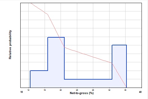 Example of Histogram Distribution shape
A histogram has two "styles". The original implementation in REP used the height of each step to represent the probability. We did it this way to make it easier to enter spikes - high probability but narrow range. This is "By amplitude". In the revised version (introduced in version 5.51e and now the default for any new histogram entry) the area of each step defines the distribution ("By area"). The advantage of the "By area" method is that if you look at the actual data used in the simulation (see Data points) it mirrors the histogram you have entered.
A general cumulative distribution in which you must enter the minimum and maximum values of the parameter, and then assign cumulative probabilities to as many intermediate values as you like. In effect, you draw the cumulative probability curve by specifying points on the line (and REP will join up the points using straight lines).
The table has two columns, probability and value. You must start with the lowest value (P100) and end with the highest (P0). For example:
Probability |
Value |
100 |
20 |
90 |
40 |
70 |
50 |
40 |
86 |
10 |
128 |
0 |
160 |
Similar to the user cumulative but a relative distribution.
The variable entry screen is similar for all probability distribution entries. You specify the shape and then enter the numbers required to define the curve.
For a rectangular distribution you enter min. and max.; for triangular, enter min., mode and max. or P90, mode and P10; for normal and log-normal enter P50 and P10 (or as otherwise specified in the program customization); for single enter the mode (which is also the min. and max.).
With triangular, normal and log-normal distributions you can change the entry style by clicking the "Style.." Button
For histograms and user distributions you must fill in the table of P levels and parameter values. For user-cum, the P levels (column Prob.) must start at 100 and decrease, and the parameter values (column Value) must increase. Click the Sort button to sort the lines into the right order.
For histogram and user relative distributions the parameter values must increase down the table but the probability levels need not. In these distributions, the probability levels are relative and need not add up to 100 (the program will adjust everything).
The graph on the right of the screen shows the distribution with the key points highlighted. You can click and drag the key points to new locations. For poly distributions double click to add new points into the curve and double-click existing points to remove them.
Note: There is often some confusion as to the meaning of minimum and maximum. Explorationists sometimes consider the minimum value of a parameter to be the one which will give the smallest result, thus the minimum value of SW when SW must lie between 20% and 45% is 45% because this will give the smallest hydrocarbon reserve.
For consistency (and to avoid confusing users working for the water companies) REP always considers the minimum value of any parameter to be the smallest numerical value that the parameter can take. In the Sw example above, the minimum Sw is 20%, because 20 is a smaller number than 45.
REP will check an entered distribution for obvious inconsistencies. It will not allow you to enter a net-to-gross ratio of less than 0% or more than 100%, for example. When entering normal and log-normal distributions REP calculates the effective P100 and P0 (see above under the description of the normal distribution) and checks that these fall within the normal parameter limits.
With the clip check box checked, the variable value is truncated between the minimum and maximum values entered. You can leave either value blank, and it is not used.
The way it works during the calculation is as follows. At each iteration, values are chosen for all the input variables according to the probability distribution (or according to the dependency relation, if a dependency is being used). If any of the variable values falls outside of the clipping limits, that iteration is discarded and new values chosen. If more than 40% of all iterations are discarded because of clipping, the calculation is stopped and a null result returned: you need to go back and revisit the distributions to reduce the amount of clipping.
The issue with clipping is that it alters the effective distribution. What you enter as the P50 (for example) will not be the P50 once the clipping has taken place. Severe clipping makes the difference important.
On the other hand, normal and log-normal distributions go on "for ever", and if you happen to be using one of these for porosity, for example, clipping to reasonable values (such as 2 - 40%) is a reasonable action.
You can enter some distributions in different ways - click the Style button to change how you do it. Styles can be different for different variables with the same shape.
Triangular and beta distributions are normally (sic) entered as minimum, mode (most likely) and maximum. But you can also enter P90, mode and P10. The value of the mode must lie between the P90 and P10 values. This is a REP requirement rather than a mathematical one. For example, in a right-angled triangle skewed to the right, the mode is less than P90. If you want to enter such a distribution into REP you must use minimum-mode-maximum.
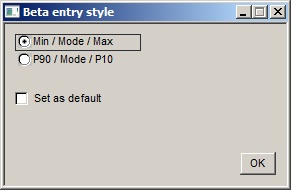
Min/Mode/Max etc. |
Choose which style you want |
Set as default |
Set the chosen style as the default for all future entries of a variable with this shape. |
Log-normal and normal distributions are specified by any two points on the distribution. The most common pairs are P50/P10, P90/P10, P90/P50 and P99/P1. But you can choose any pair you like. Click the style button to show the dialog:
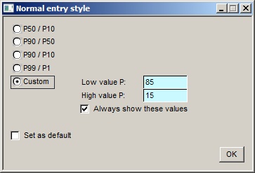
P50/P10 etc. |
Choose which style you want. [Note: There is an increasing body of opinion that holds that you should use the P99 and P1 to enter normal and, particularly, log-normal distributions. This is because it is considered difficult for most people to estimate "central" values correctly; an absolute minimum (P99) and an absolute maximum (P1) are more readily and accurately quantified. A number of experimental studies are said to confirm this hypothesis. It must be said that this theorem is not obviously true and I am grateful to Dr Mike Treesh, an expert in this field, for the trenchant observation that if you want to determine the average height of a population you do not go hunting for the shortest and tallest people in it, for very obvious reasons.] |
Custom |
If you choose this one, enter the two P levels you want to enter. "Low value" and "High value" refer to the variable value, so the "Low value P" is the probability level of the low variable value, the "High value P" the probability level of the high variable value. The P level of the low value should be greater than the P value of the high value. Obviously. Either of these custom P values can be one of the standard ones - i.e. 99, 90, 50, 10 or 1. So you could use P50/P15. |
Always show these values |
Check this to show the custom P values on the entry dialog, even if you are using one of the pre-set styles. |
Set as default |
Set the chosen style as the default for all future entries of a variable with this shape. |
It is possible to copy a distribution to another prospect or model. See 'Copying Distributions to Other Models or Prospects' for more information.