Gross rock volume

There are three methods for entering gross rock volume (GRV): as a single distribution, as the product of area, thickness and shape factor and from area/depth (contour maps) (you can also enter GRV/depth data or net pay maps).

A single distribution is appropriate where the numbers are coming from - or are based on - the results of a mapping or geological modelling program. Area/thickness/shape should be used either when the thickness of the reservoir is small compared to the closure (and the structure is fairly flat) or when no detailed structural data are available - normally very early on in the prospect appraisal process.

If the data are available it is best to use the area/depth entry, since this allows proper appreciation of the errors in the mapping process.

A GRV multiplier known as the stacking factor can be applied.

See 'Entering Probability Distributions' for help with probability distributions.

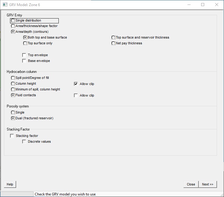
GRV Entry	Check the GRV model you wish to use - see above. If you choose Area/depth then you need to specify what configuration you want:
Define both top and base surface	This is especially useful for stratigraphic traps.
Define a top surface and reservoir thickness	A common case where the base of the reservoir conforms with the top of the reservoir.
Define a top surface only	Used where the thickness of the reservoir is always greater than the structural closure (i.e the thickness is greater than any anticipated column height)
Define a net pay thickness	Here the contours on the map represent net pay thickness.

Hydrocarbon column	Given a structure, REP needs to know how much of it is filled with hydrocarbon. You can define the base of the hydrocarbon column either as a column height (extent from the crest of the structure) or as a depth - either a spill point or a fluid (hydrocarbon/water) contact. In terms of the calculation there is no difference between a spill point and a hydrocarbon contact unless you are going to use surface shifts, in which case the difference is important. Spill points shifts with the top surface, so if you have a surface shift and no base reservoir there will be no net change in reserve. But contacts are assumed fixed in depth, so there will be a change as you shift the top surface. In the case of column height, you can "Allow clip". Normally if you set a clipping limit on a variable, and in a calculation iteration that limit is exceeded, the iteration is discarded. Allowing the clip sets the column height value to its clipping value and allows the iteration to proceed. This of course will give you more hydrocarbon. Another way to achieve a similar end is to define both a spill point and a column height. In this case REP will randomly choose values for both (in the usual way) and choose the minimum of the two. Degree of fill is not used.

Porosity Model	In a single porosity model there is one porosity, net-to-gross, Sw and recovery factor - this is the usual case. In a dual porosity model you have two sets of porosity, net-to-gross, Sw and recovery factor. Commonly this is used for fractured reservoirs,(and the secondary porosity is called Por (fr), similarly Sw (fr) etc.); but the "secondary" porosity could just be another facies. In the case of fractured reservoirs, it is usual to put the fracture recovery factor to 100%, and the Sw to 0%. This is defensible, especially in a REP context. That leaves porosity and NTG: you have to manipulate these to get the volumes about right. Some people put porosity=100% and adjust the NTG so that it approximates a fracture density that they can derive from image logs. Others do the opposite - they put NTG=100% and enter an overall fracture porosity. It doesn't really matter, as long as the numbers are reasonable. The disadvantage of the latter method is that the back-calculated average net-to-gross and therefore net thickness are nonsense, even of the volumes are right. Consider a case where the matrix porosity of (for example) 4%. The two porosity systems sit side-by-side so the average NTG is now >100%, and net thickness > gross thickness. For this reason it is recommended in fractured reservoirs to use a low fracture NTG and if necessary high porosity. Note that fractured reservoirs are tough to analyse at the best of times, and REP is not an expert in the field. One of our early users suggested that the output sheets for fractured reservoirs should have the banner "Sell!" across them. Perhaps he was right.

Stacking factor	Check to apply stacking factor. This is a simple gross rock volume multiplier and can be useful when you are dealing with plays with multiple pays. You enter the stacking factor as a variable in the normal way. Effectively you are saying: I have modelled a sand, and I have 6 or 20 or 47 just like it.
Discrete values	REP variables are continuous, which in the case of stacking factor means that (for example) a value of 6.778 could be chosen for a given iteration. Obviously stacking factor should really be a whole number, and checking this box means that on any given iteration the chosen number is rounded up or down to the nearest integer (7, in this case). The difference in the calculated results will be very small, but it may make you feel better.

Single Distribution

GRV is entered as one distribution. The units are acre-ft or mmcm (km2-m).

The problem with using a single distribution is that there is no depth information, so you cannot model uncertainty in hydrocarbon contacts, thief zones, gas columns etc.. These are all wrapped up in the single distribution. This is a pity, since GRV is usually the single biggest source of uncertainty.

Area/Thickness/Shape Factor

GRV is the product of three distributions: area, thickness and shape factor. The shape factor is a correction factor to account for edge and other geometrical effects when using the area/thickness model. Figure 1 shows a table of shape factors for dome/pyramid and prism/cylinder reservoir geometries. Enter the chart on the left with the approximate ratio of reservoir thickness to closure height, go across to the line which best describes the geometry, and then down to read the shape factor multiplier. Be aware that the shape factors are approximate (your structure is unlikely to have been laid down either by an Egyptian Pharaoh or the late Mr. Christopher Wren) and introduce a notable source of error just by themselves; also, the shape factor is de facto dependent on the reservoir thickness.

If the reservoir thickness is very small compared to closure, then the shape factor is nearly 1.0, and the method can be used with acceptable accuracy. And if your source data are just a few speculative areas on a geographical map the method may be the only one you can use. But as soon as you can start using a proper map and enter area/depth data, do so!

Figure 1 - Reservoir shape factors.

Contour Maps

Entry from contour maps (actually area/depth or GRV/depth data pairs) is a bit more complicated but allows much more flexibility. There are three forms of entry:

1. Top and base horizons

2. Top horizon and reservoir thickness

3. Top horizon only

4. Net pay maps

A mapped horizon is one for which you enter the contours and associated areas. It may or may not correspond to the top or base of the reservoir. (See surface shifts below).

The area/depth details of each horizon may be entered in the Surface Entry screen, or read from a file. In the latter case the file should be prepared using the Map Digitization Module.

[Note: If changes are made to the .srf file in the Maps module, then the filename (at the bottom of the dialog) will turn red and should be reloaded using the re-load button.]

pr-grv2

File menu
Load surface file	Click to browse for a new surface file and load the area/depth data
Import	Click to import data. The data should be an ASCII text file, either space, tab or comma delimited.

Area/GRV
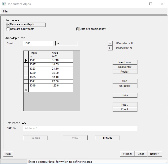
Data are area/depth	The data can be either area/depth or GRV/depth. See Area vs. GRV below. You can also work from net pay maps ("area/net pay"), though this is not recommended.

Area/depth table
Crest	This is the highest point of surface - with a zero area.
Depth	Enter a contour level for which to define the area
Area	Enter the area associated with this contour

Buttons
> Ft acre; >m/km2	Two buttons that quickly let you change the units (values are converted)
Insert row	Click to insert new row above selection
Delete row	Click to delete selected row
Restart	Click to delete all contours and start again
Sort	Click to sort the contours in depth order
Un-petrel	When pasting area/depth from Petrel, the depths usually come in as negative values, and in reverse order. Clicking this button will reverse the sign of the depths (negative becomes positive and vice-versa) and the order becomes shallow to deep deep. Think of this button as changing your world from a cup half empty to a cup half full.
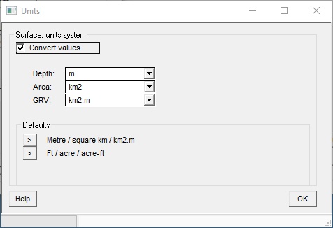
Units	Opens a dialog where you can change the units.
Plot ..	Click to draw the area/depth (or GRV/depth) graph
Check	Check the data for inconsistencies (wrong order etc.)

Data loaded from
SRF file	Specifies location of surface data, The surface data (srf file) is produced when you use REP's map digitisation module.
Re-load	Click to reload the data from the specified surface file. If the data in the srf file have been changed since you last loaded them here this entry is red.
View	Click to view the map image file
Browse	Click to browse for a new surface file and load the area/depth data

Using the Surface Entry screen, the area depth numbers are entered directly into a table. You should think of the table as a numerical representation of the area/depth or GRV/depth plot. Each horizon has a crest (its highest point - the depth with zero area) and then contour levels with associated areas.

In the table, contour levels and areas (or GRV's) should both increase down the table.

You can paste in numbers from the clipboard. First copy the numbers into the clipboard from XL or any other compliant program, then press Ctrl-v on the keyboard to paste. If there are two columns in the clipboard they will fill the table. You can also paste column-by-column, by first clicking in the REP column you want to populate.

You can also import the data from a text file.

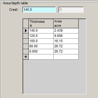
If your map is of net pay thickness, then the "crest" should be the maximum net pay thickness (with a zero area) and the "thickness" refers to net pay thickness and should decrease down the table, as the area increases. Here's an example:

pr_grv3

Area vs. GRV

If you have area data, and flick from area input to GRV input, the program will calculate the GRV at each contour depth and present this in the table. And vice-versa. (If you already have data calculated or entered, you are prompted before it recalculates the numbers.)

But it is important to appreciate that although the conversion is exact, choosing to calculate using area/depth may give a slightly different answer to that using GRV/depth. It is not much - it depends on how many depths you have entered - at worst a few percent. This is not a bug. It happens because, for depths between the contour levels, the program interpolates the data. Interpolation in the area domain gives slightly different results to interpolation in the GRV domain.

Area/GRV/depth units

This dialog lets you change the units. By default any existing data will be converted to the new units. If you don't want to do this un-check the "Convert units" check box. This is particularly useful when pasting in data. You sometimes find that - in your excitement - you've forgotten to pre-set the units correctly.

pr_ardunits

Surface shifts

Having entered the top horizon, you are prompted for the surface shifts (if any).

The displacement from a mapped horizon to a reservoir surface is entered as a shift (which may be a constant or a probability distribution). In REP, a positive shift is a shift downwards (increasing depth). Figure 2 shows the relationship between a mapped horizon and the reservoir top surface, where the mapped horizon is below the reservoir - so the shift (marked 1) is negative. In figure 3 the mapped horizon is above the reservoir, so the shift (1) is positive. You may also define a shift from the top reservoir to the base seal (marked 2 in figures 2 & 3).

Figures 2 & 3 - The relationship between mapped horizon and reservoir surfaces.

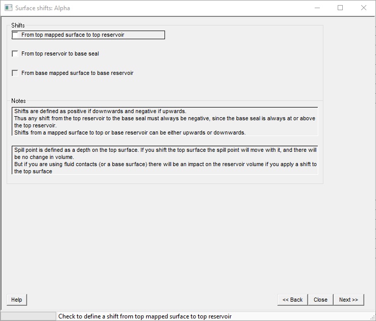
Shifts
From top mapped surface to top reservoir	Check to define a shift from top mapped surface to top reservoir
From top reservoir to base seal.	Check to define a shift from top mapped surface to base seal. You use this if you have a "thief zone" at the top of the reservoir. It is exactly equivalent to moving the spill point up by the thickness of (shift to) the thief zone.
From base mapped surface to base reservoir	Check to define a shift from base mapped surface to base reservoir
Notes
Notes	-

These relate:

(a) the top horizon to the top reservoir

(b) from the top reservoir to the base seal

In REP, a negative shift is a shift upwards (decreasing depth) and a positive shift is a shift downwards (increasing depths).

[Note: Shift (b) above is from the top reservoir and not from the top horizon. Therefore, this shift is always negative since the base seal is assumed to be above the top reservoir. Also, note that the minimum value of the shift must always be a bigger negative number than the maximum shift. This is because, to REP, the minimum value is always, numerically, the smallest: for example, -80 is less than -35.]

Also related to the top horizon is the spill point. This is entered as a depth on the top horizon. The program will adjust the depth to the appropriate reservoir depth when it does the calculations.

If you have entered a base horizon you may specify a shift from it to the base reservoir.

REP makes a number of checks on the integrity of the horizon entry. In particular it checks that the base of the reservoir is below the top of the reservoir, and that the spill points and contact levels lie within defined depths on the area/depth curve. However, with all entries being distributions, and the possibility of so many shifts, the number of possible combinations is very large. Final responsibility for data entry is with you the user. It is always advisable to view or print the area/depth curve to check that no error has crept in.

Area Uncertainty

Area uncertainty is a simple multiplier to account for errors in the contouring - essentially, at any depth, it says that the area could be larger or smaller by a given amount (the error is - of course - entered as a probability distribution).

(Note than in earlier version of REP you had the choice to define or not an area uncertainty. Now you always have it.)

Stacking Factor

Whatever form of GRV entry you have chosen you can enter a stacking factor. A stacking factor is useful in plays with multiple pays. REP treats the stacking factor as a simple multiplier in the GRV calculation. Not specifying a stacking factor is equivalent to defining one with a single value of 1.0.

A typical use of the stacking factor is where there are a number of separate but presumably similar sands each with its own fluid contact. The rigorous way to handle this would be to model each sand separately and then consolidate them. But if there are lots of them this is time-consuming and very possibly pointless. Take one (or perhaps a couple of groups) and then apply the stacking factor to multiply up by the number of them that there are. Note that the stacking factor can account not only for the number of them, but also for variations between them.

By default the stacking factor is a continuous distribution. If you check "Discrete values" you force the stacking factor to take only integer (whole) numbers, with a minimum value of 1. This doesn't make much difference to the result, unless the distribution is small and tight.

Where there is (or may be) a change in some property with depth (which presumably also equates to the number of them) you can use dependencies to model that change. Examples of such a dependent property are porosity and formation volume factor.